Multidimensional Chromatography

90	Multidimensional Chromatography

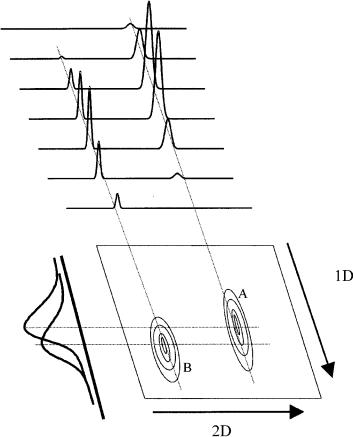
Figure 4.8 The GC GC experiment can be considered to be a series of fast second chromatograms conducted about five times faster than the widths of the peaks on the first dimension. The 1D elution time is the total chromatographic run time, while the 2D time is the modulation period (e.g. 4 – 5 s). This figure shows two overlapping peaks A and B, with the zones of each peak collected together. When these slices are pulsed to the second column, they are resolved. Here, we show peak B eluting later on column 1, but earlier on column 2, with the 2D peak maxima tracing out a shape essentially the same as the original peak on 1D.

column 2 (e.g. using a more selective stationary phase) then each peak becomes a series of related second-column peaks. These secondary peaks will increase and then decrease according to how the primary peak distribution varies on the first column. Note that peak B has a longer retention time tR on column 1, but is drawn as a shorter tR on column 2. This would suggest that compound B has a smaller distribution coefficient (K) than compound A on column 2, and consequently a smaller retention factor, k, and thus a smaller retention time than A.

The peaks are revealed in the 2D separation space as oval-shaped peaks in a contour plot format, reproduced as a schematic diagram in Figure 4.9. The contour peaks are now completely separated in the 2D space, whereas they were severely overlapping on the first column.

This novel manifestation of the gas chromatographic separation demands that our fundamental understanding of the GC method – invariably of single-dimensional scope – is challenged as follows: concepts of column efficiency and separation are now supplanted by a need to compare the performances of two columns operating

Orthogonal GC–GC

91

Figure 4.9 The peaks produced in the second dimension (see Figure 4.8) can be plotted as a contour shape in the retention or separation space, with characteristic retentions in each dimension. It can be seen that such peaks are now well resolved.

simultaneously; the usual post-run simple method reports are no longer simple since we have multiple peaks reported in the analytical results of a chromatogram for every single peak in a sample and recombining these back to the one component for purposes of quantitation are required; even retention is not an easy property to define because it will relate to the modulation period in addition to the first-column retention. These are, however, challenges which clever programming and familiarity with chromatogram interpretation will resolve in time. At present, the state-of-the- art of GC GC appears to be in its qualitative capabilities. Selected highly complex samples have been reported in the GC GC experiment, chiefly in the petroleum area – few other samples can be as complex as these – and the general consensus is that GC GC has revealed complexity that has never before been realized, even though it may have been suspected. Not only have the samples been

92	Multidimensional Chromatography

pulled apart in the 2D space, but even minor or trace components that would never have been exposed in the single column are often clearly placed as fully separated peaks.

The fact that we have peaks within a 2D space implies that where no peak is found represents a true detector baseline or electronic noise level. In a conventional petroleum sample, a complex unresolved mixture response causes an apparent detector baseline rise and fall throughout the GC trace. It is probably a fact that in this case the true electronic baseline is never obtained. We have instead a chemical baseline comprising small response to many overlapping components. This immediately suggests that we should have more confidence in peak area measurements in the GC GC experiment.

4.3.4 CONSIDERATIONS OF RETENTION ON THE SECOND COLUMN – WRAPAROUND

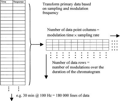
For unresolved peaks eluting from the first column into the modulator, each pulsed solute packet delivers a group of components to column 2. It does this every modulation event, e.g. every 4 s. There is no guarantee that each solute will have a retention less than the modulation time, and so some peaks may not have reached the detector by the time the next packet of solute is launched into the short fast second column. The procedure for generation of the matrix format is illustrated in Figure 4.10. The column data are taken in blocks of data points equal to the number of points corresponding to the modulation time, and put into a column. This procedure is repeated until the full data are transformed. If a peak from one modulation event happens to be retained longer than the sampling period, then it will not be included in that period’s transformed data block. Let us say the solute has a 2D retention time of 5 s. Since the data are transformed into matrix form for 2D presentation, using the 4 s modulation time as one matrix edge, then the 5 s retained solute will have an apparent transformed time of 1 ( 5 4) s, and its peak will appear to be centred on a time of 1 s in the 2D plot. Thus, while we normally use the labels ‘first dimension retention’ (which is correct) and ‘second dimension retention’ for the 2D space, the above solute does not have an absolute retention of 1 s on the second column. (It may be more appropriate to say ‘apparent retention’ or use a similar term to reflect that the time does not necessarily have an absolute meaning on the 2D axis.) Here, the solute has ‘wrapped around’ one set of matrix transformations of data and so appears in the subsequent matrix data line. It is possible to have solutes wraparound more than once. A useful way to decide if wraparound occurs is to study peak widths in the second dimension. Those peaks retained more will have increasingly wide peaks. In a recent study, for instance, of derivatized sterols (24), the high elution temperature meant that the sterols eluted during the isothermal hold period (at 280°C). Thus, the later peaks not only became increasingly broad in the first dimension, but because they were less volatile they were more retained on the second column. A modulation of 4 s was used, and the last sterol had a 2tR time of

Orthogonal GC–GC

93

Figure 4.10 Representation of the transformation of data from a single-column data string to a matrix form, based on the sampling frequency and modulation time. The data points acquired for each modulation period are placed in a separate row of the matrix. The matrix data are then in a suitable format to read into an appropriate plotting package such as the ‘Transform’ program.

about 11 s, indicating that it was ‘wrapped-around’ twice. The sterol was located at 3 s in the 2D space, i.e. two wraparounds 8 s, plus 3 s. The first eluting sterol had a 2tR time of about 3 s, while the others had 2tR times of about 4, 6 and 7 s as their retentions increased. The latter two peaks therefore appeared in the 2D space at about 2 s and 3 s. If the sterols were eluted during the temperature programme ramp, they would appear with a relatively constant 2tR time, since the decreasing volatility of the later sterols are compensated by the increased temperature at which they enter the second column.

In a novel experiment where a programmable temperature vaporizer (PTV) injector was used to continually supply dodecane sample into the first column, and presenting the retention on the second column for the dodecane during a temperature programmed analysis, it was possible to generate an isovolatility line for the second column which looked somewhat like a long tail extending through the separation space (26). Its retention decreased as the oven temperature increased, as was predicted. In some studies, in contrast, stationary phase bleed does not seem to trace out such a retention reduction. Presumably, since bleed comprizes highly volatile

94	Multidimensional Chromatography

solutes, and only occurs at reasonably high oven temperature, it behaves almost as an unretained solute. In this case, the bleed retention profile may reflect the change in carrier gas flow in the second column as the temperature increases.

4.4ORTHOGONALITY OF ANALYSIS

Multidimensional analysis methods rely on exploiting different properties or responses of solutes based on more than one physical/instrumental process, normally operated in series. Thus, a separation dimension coupled with a spectroscopic dimension constitutes a multidimensional analysis (27). The usual value of such a method is that if components are not uniquely identified in one dimension, then they will hopefully be identified in the second. Provided that the response bases of both dimensions are sufficiently different, then an orthogonal analysis results. If the mechanism of the two dimensions are similar, then we might propose that some degree of correlation exists, and this may reduce the identification power of the multidimensional analysis. For example, HPLC – diode array detection (DAD) can be regarded as orthogonal two-dimensional analysis because there is no correlation between the HPLC retention and the UV spectra of the components. Cortes has discussed a variety of coupled separation dimensions involving different chromatographic modes (28). An HPLC – high resolution GC system will likewise be orthogonal (29), and has been applied to such diverse applications such as oil fractions (30) and food and water analyses (31). The HPLC – capillary electrophoresis experiment involves two separation dimensions, but solutes respond in each dimension differently – HPLC according to the distribution constant of solutes between the mobile and stationary phases, and CE according to electrophoretic mobility (arising from solute size-to-charge properties). We might then conjecture that a multidimensional experiment employing reversed-phase HPLC and capillary electrochromatography on a non-polar phase material may possess a degree of correlation, since there will exist retention parameters strongly dependent upon partitioning processes into the reversed-phase stationary material which is common to both dimensions. In contrast, for the HPLC–DAD analysis the specificity of analysis then relies upon the components having uniquely identifiable or assignable spectra.

The most valuable tool for routine orthogonal two-dimensional analysis in GC is the GC – MS technique, with the dimensionality being shown schematically in Figure 4.11(a) for a GC – MS system where compound identity is defined by its time on the column (1D) and mass spectra (2D). Choosing unique or characteristic ions for overlapping components can produce reliable quantitative estimations of each component. How do we extend this argument to gas chromatography? In GC, MDGC is a two-dimension separation method. We might initially suggest that since we have two GC dimensions, then they must be correlated. However, the two dimensions will not be correlated provided that the mechanism of interaction between the components of a mixture and each column is different. Clearly, two columns of the same phase type operated at the same temperature will be correlated, and two components overlapping on the first column will not be expected to be separated on the

Orthogonal GC–GC

95

Figure 4.11 (a) Representation of GC – MS as a two-dimensional analysis method. (b) Representation of GC GC as a two-dimensional separation, with separation mechanisms based of different chemical properties in each dimension.

second. We gain no extra separation or identification information from this experiment; there is no orthogonality. Thus, we ensure orthogonality of an analysis by employing techniques which exploit the chemical properties of the solutes to be studied, in a manner that gives independent responses in the two dimensions. In the case of two separation dimensions, we can force orthogonality by varying the analysis conditions of the second separation dimension as the first dimension proceeds. This can be referred to as tuning of the conditions, and is essentially achieved by using a second temperature zone for the second column.

4.4.1 HOW CAN WE ENSURE THAT THE TWO COLUMNS ARE ORTHOGONAL?

The elution of compounds on GC columns is a complex process related to the volatility of the compound, which results from its boiling point, and the chemical interactions between the compound and the stationary phase. These interactions are typically those which arise from polar – polar interactions, dispersion forces, dipole – dipole interactions, and so forth. Collectively, they are described by the term the chemical potential, °, which derives from the potential for the compound to

96	Multidimensional Chromatography

be transferred from the mobile to the stationary phase. This then alters the distribution constant and also the retention factor (i.e. retention time) of the compound. If two compounds have the same chemical potential on one column, then in order to separate them in a multidimensional experiment we have to alter their chemical potentials. This can be done by using a different temperature on the two dimensions, although a more useful approach is readily achieved by choosing different stationary phase types. Figure 4.11(b) shows that the first dimension separates by the property of volatility, and the second by polarity. The response axis indicates the detector response to the solute. Temperature variation on the two columns is a less practical solution, since we require two independently controllable temperature regions – such as a two-oven system. Most studies of multidimensional gas chromatography employ different column phases, and as a typical example we can consider a hypothetical experiment of a processed petroleum (e.g. kerosene) sample separation.

To a first approximation, the analysis of the petroleum sample on one stationary phase column versus another column will to a large extent appear very similar. The chromatogram will be dominated by the saturated alkanes, with the normal hydrocarbon suite providing the recognizable dome shape. Between the major components will be a range of branched and aromatic compounds. We cannot distinguish these minor components due to the large number of overlapping components, and one column is unlikely to be very much better than another. Admittedly, with mass spectral detection, we might be able to say that one column gives a better result than the other, but with flame-ionization detection the complexity is overwhelming. Different phases will shift the peak relative retentions, but for the kerosene trace components this is a little like changing one scrambled chromatogram for another. Each column separates or retains (primarily) by the component boiling point, and then imposes a selectivity or relative peak position adjustment based on what we might call polarity, but is better referred to as specific solute – stationary phase interactions.

With comprehensive GC, we can now choose a rational set of columns that should be able to ‘tune’ the separation. If we accept that each column has an approximate isovolatility property at the time when solutes are transferred from one column to the other, then separation on the second column will largely arise due to the selective phase interactions. We need only then select a second column that is able to resolve the compound classes of interest, such as a phase that separates aromatic from aliphatic compounds. If it can also separate normal and isoalkanes from cyclic alkanes, then we should be able to achieve second-dimension resolution of all major classes of compounds in petroleum samples. A useful column set is a low polarity 5 % phenyl polysiloxane first column, coupled to a higher phenyl-substituted polysiloxane, such as a 50 % phenyl-type phase. The latter column has the ability to selectively retain aromatic components.

The concept of tuning a separation was succinctly summarized by Venkatramani et al. who stated (32):

A properly tuned comprehensive 2-dimensional gas chromatograph distributes substances in the first dimension according to the strength of their dispersive interactions . . . and in the second dimension according to their specific non-dispersive

Orthogonal GC–GC

97

interactions . . . independent of any dispersive interactions the two stationary phases may have in common.

This statement refers to a non-polar first column and a more polar second column.

The ordering of classes of compounds within the separation space was summarized by Ledford et al. (33), who presented an analogy to the separation by using a mixture of objects of varied shapes, colours and sizes. The experimental dimensions could separate objects based on mechanisms which were sensitive to shape, size or colour, and the choice of two of these for the two-dimensional separation was illustrated. Applications showed a variety of petroleum products on different column sets, as well as a perfume sample.

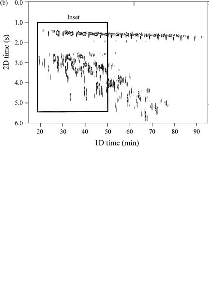
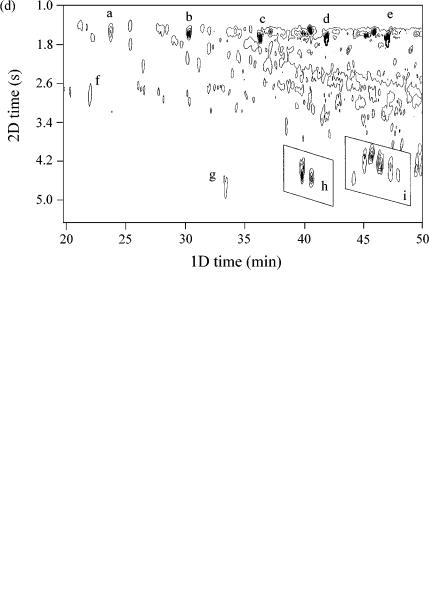
Figure 4.12 is an example of such a separation obtained from work in our laboratory. Figure 4.12(a) shows a surface response plot which is reproduced in Figure 4.12(b) as a contour plot. The sample used is a light cycle oil, which has had certain components (presumably cyclic alkanes) removed through reforming the oil. Thus, there is a vacant region in the 2D space between the linear and branched alkane peaks (located at a 2D time of 1.5 – 2.0 s), and aromatic solutes (benzenes, naphthalenes, etc., located from 2.5 – 6.0 s). The aromatic solutes are more polar and interact more strongly with the BPX50 stationary phase so are retained longer than the saturated compounds on the second column. The inset region of Figure 4.12(b) is expanded and shown in Figure 4.12(c). The linear alkanes are identified as peaks ( a ) – (e), with some selected other peaks (f), (g) and the groups (h) and (i) also being shown on this trace. Figure 4.12(d) shows the data obtained for a light gas oil, which has not been treated to remove the components noted as being absent in Figure 4.12(c). The same analysis conditions were used, and the same inset expansion is used for both of these figures. The same solutes ( a ) – (i) are identified in Figure 4.12(d), and the almost exact correspondence of these peaks is evident.

While samples such as these have obviously been the focus for much GC GC work in the past, the technology still remains to be demonstrated for many other sample types. It is likely that in the near future, as many more applications are studied, a general theory – or at least a guide to column selection for GC GC applications – will reveal a logical approach to selection of phases that embodies the principles of orthogonality of separation.

As a further example, we have recently completed one of the first studies of complex essential oil analysis by using GC GC methods (34). While for petrochemical (35) and semivolatile aromatic compound analysis (36), we found the column set BPX5 – BPX50 to be excellent – with the latter column able to separate saturated compounds from aromatics that coeluted on the first column – the nature of essential oil composition is such that we do not require the tuning of an aliphatic/aromatic separation, but rather we require a non-oxygenated/oxygenated component separation (with some degree of unsaturation also useable for separation). The obvious choice is a polar poly(ethylene glycol) column as the second dimension. Figures 4.13 and 4.14 show some typical results obtained for vetiver oil on BPX5 – BPX50 and BPX5 – BP20 column sets, respectively. Note that the

98	Multidimensional Chromatography

Figure 4.12 (a) Surface response plot of a light cycle oil analysed by GC GC. The column set was a BPX5 – BPX50 combination, with the second column being 0.8 m in length. A 6 s modulation time was used, in conjunction with a 1°C/min temperature programme rate. The cycle oil has been reformed to remove the cyclic alkanes. (b) The same data as in (a), but presented as a contour plot in this case.

Orthogonal GC–GC

99

Figure 4.12 (continued) (c) An expansion of the inset region from (b), with the normal alkanes shown as (a – e). Other unidentified components (f – i) are presented to locate specific peaks for comparison purposes. (d) A light gas oil analysed under the same conditions as for the cycle oil, showing the same expanded region. In this case, the oil has not been treated in the same manner as the cycle oil, so it retains the components that were absent from the cycle oil. Peaks (a – i) are the same as those seen in (c).