812 Chapter 18 RECURSIVE PROGRAMMING

Basic Concepts

Recursive programming is used for implementing algorithms, or mathematical definitions, that are described recursively, that is, in terms of themselves. A recursive definition is implemented by a procedure that calls itself; thus, it is called a recursive procedure.

Code that calls functions and subroutines to accomplish a task, such as the following segment, is quite normal:

Function MyPayments() { other statements }

CarPayment = CalculateCarPayment(Interest, Duration) HomePayment = CalculateHomePayment(Interest, Duration) MonthlyPayments = CarPayment + HomePayment

{ more statements } End Function

In the preceding code, the MyPayments() function calls two functions to calculate the monthly payments for a car and home loan. There’s nothing puzzling about this piece of code because it’s linear. Here’s what it does:

1.The MyPayments() function suspends execution each time it calls a function (the CalculateCarPayment() and CalculateHomePayment() functions).

2.It waits for each function to complete its task and return a value.

3.It then resumes execution.

But what if a function calls itself? Examine the following code:

Function DoSomething(n As Integer) As Integer

{other statements } value = value - 1

If value = 0 Then Exit Function newValue = DoSomething(value)

{more statements }

End Function

If you didn’t know better, you’d think that this program would never end. Every time the DoSomething() function is called, it gets into a loop by calling itself again and again, and it never exits. In fact, this is a clear danger with recursion. It’s not only possible but also quite easy for a recursive function to get into an endless loop. A recursive function must exit explicitly. In other words, you must tell a recursive function when to stop calling itself and exit. The condition that causes the DoSomething() function to end is met when value becomes zero. If the initial value of this variable is negative, the function will never end, because value will never become zero. This is a typical logical error you must catch from within your code.

Apart from this technicality, you can draw a few useful conclusions from this example. A function performs a well-defined task. When a function calls itself, it has to interrupt the current task to complete another, quite similar task. The DoSomething() function can’t complete its task (whatever this is) unless it performs an identical calculation, which it does by calling itself.

Copyright ©2002 SYBEX, Inc., Alameda, CA

www.sybex.com

BASIC CONCEPTS 813

Recursion in Real Life

Do you ever run into recursive processes in your daily tasks? Suppose you’re viewing a World Wide Web page that describes a hot new topic. The page contains a term you don’t understand, and the term is a hyperlink. When you click the hyperlink, another page that defines the term is displayed. This definition contains another term you don’t understand. The new term is also a hyperlink, so you click it and a page containing its definition is displayed. Once you understand this definition, you click the Back button to go back to the previous page where you re-read the term, knowing its definition. You then go back to the original page.

The task at hand involves understanding a topic, a description, and a definition. Every time you run into an unfamiliar term, you interrupt the current task to accomplish another identical task, such as learning another term.

The process of looking up a definition in a dictionary is similar, and it epitomizes recursion. For example, if the definition of an ASP page is “ASP pages are Web pages that contain Web controls,” you’d probably have to look up the definition of Web controls. Once you understand what Web controls are, you can go back and understand the other definitions. Let’s say that Web controls are defined as “elements used to build ASP Web pages.” This is a sticky situation, indeed. At this point, you’d either have to interrupt your search or look up its definition elsewhere. Going back and forth between these two definitions won’t take you anywhere. This is the endless loop mentioned earlier.

Because endless loops can arise easily in recursive programming, you must be sure that your code contains conditions that will cause the recursive procedure to stop calling itself. In the example of the DoSomething() function, this condition is as follows:

If value = 0 Then Exit Function

The code reduces the value of the variable value by increments of 1 until it eventually reaches 0, at which point the sequence of recursive calls ends (provided the initial value of the variable is positive, because if you start with a negative value you’ll never reach zero). Without such a condition, the recursive function would call itself indefinitely. Once the DoSomething() function ends, the suspended instances of the same function resume their execution and terminate.

When you interrupt a task to perform another similar task, you’re performing some type of recursion. Each new task in the process involves a different definition, but the goal is to gather all the information you need to complete the initial task. Now, let’s look at a few practical examples and see these concepts in action. The first example is a trivial one, but you’ll be able to follow the thread of recursive calls and understand how recursion works. In the following sections, we’ll build more difficult, and practical, recursive procedures.

A Simple Example

I’ll demonstrate the principles of recursive programming with a simple example: the calculation of the factorial of a number. The factorial of a number, denoted with an exclamation mark, is described recursively as follows:

n! = n * (n-1)!

The factorial of n (n!, read as “n factorial”) is the number n multiplied by the factorial of (n – 1), which in turn is (n – 1) multiplied by the factorial of (n – 2) and so on, until we reach 0!, which is 1 by definition.

Copyright ©2002 SYBEX, Inc., Alameda, CA

www.sybex.com

814 Chapter 18 RECURSIVE PROGRAMMING

Here’s the process of calculating the factorial of 4:

4! = 4 * 3!

=4 * 3 * 2!

=4 * 3 * 2 * 1!

=4 * 3 * 2 * 1 * 0!

=4 * 3 * 2 * 1 * 1

=24

For the mathematically inclined, the factorial of the number n is defined as follows:

n!	=	n * (n-1)!	if	n	is	greater than zero
n!	=	1	if	n	is	zero

The factorial is described in terms of itself, and it’s a prime candidate for recursive implementation. The Factorial application, shown in Figure 18.1, lets you specify the number whose factorial you want to calculate in the box on the left and displays the result in the box on the right. To start the calculations, click the Factorial button.

Figure 18.1

The Factorial application

Here’s the Factorial() function that implements the previous definition:

Function Factorial(n As Integer) As Double

If n = 0 Then

Factorial = 1

Else

Factorial = n * Factorial(n - 1)

End If

End Function

The recursive definition of the factorial of an integer is implemented in a single line:

Factorial = n * Factorial(n-1)

As long as the argument of the function isn’t zero, the function returns the product of its argument times the factorial of its argument minus 1. With each successive call of the Factorial() function, the initial number decreases by an increment of 1, and eventually n becomes 0 and the sequence of recursive calls ends. Each time the Factorial() function calls itself, the calling function is suspended temporarily. When the called function terminates, the most recently suspended function resumes execution. To calculate the factorial of 10, you’d call the Factorial() function with the argument 10, as follows:

MsgBox(“The factorial of 10 “ & Factorial(10))

The execution of the Factorial(10) function is interrupted when it calls Factorial(9). This function is also interrupted when Factorial(9) calls Factorial(8), and so on. By the time Factorial(0) is called, 10 instances of the function have been suspended and made to wait for the function they

Copyright ©2002 SYBEX, Inc., Alameda, CA

www.sybex.com

BASIC CONCEPTS 815

called to finish. When that happens, they resume execution. The first instance to resume its execution is the Factorial(1), then the Factorial(2), and so on.

Let’s see how this happens by adding a couple of lines to the Factorial() function. Open the Factorial application and add a few statements that print the function’s status in the Output window, as shown in Listing 18.1.

Listing 18.1: The Factorial() Recursive Function

Function Factorial(n As Integer) As Double Console.WriteLine(“Starting the calculation of “ n & “ factorial”) If n = 0 Then

Factorial = 1 Else

Console.WriteLine(“Calling Factorial(” & n – 1 & ”)”) Factorial = Factorial(n - 1) * n

End If

Console.WriteLine(“Done calculating “ & n & “ factorial”) End Function

Watching the Algorithm

You can watch the execution of the algorithm by inserting a few statements that display the progress on the Output window (the WriteLine statements in Listing 18.1). The first WriteLine statement tells us that a new instance of the function has been activated and gives the number whose factorial it’s about to calculate. The second WriteLine statement tells us that the active function is about to call another instance of itself and shows which argument it will supply to the function it’s calling. The last WriteLine statement informs us that the factorial function is done. Here’s what you’ll see in the Output window if you call the Factorial() function with the argument 4:

Starting the calculation of 4 factorial

Calling Factorial(3)

Starting the calculation of 3 factorial

Calling Factorial(2)

Starting the calculation of 2 factorial

Calling Factorial(1)

Starting the calculation of 1 factorial

Calling Factorial(0)

Starting the calculation of 0 factorial

Done calculating 0 factorial

Done calculating 1 factorial

Done calculating 2 factorial

Done calculating 3 factorial

Done calculating 4 factorial

This list of messages is lengthy, but it’s worth examining for the sequence of events. The first time the function is called, it attempts to calculate the factorial of 4. It can’t complete its operation

Copyright ©2002 SYBEX, Inc., Alameda, CA

www.sybex.com

816 Chapter 18 RECURSIVE PROGRAMMING

and calls Factorial(3) to calculate the factorial of 3, which is needed to calculate the factorial of 4. The first instance of the Factorial() function is suspended until Factorial(3) returns its result.

Similarly, Factorial(3) doesn’t complete its calculations because it must call Factorial(2). So far, there are two suspended instances of the Factorial() function. In turn, Factorial(2) calls Factorial(1), and Factorial(1) calls Factorial(0). Now, there are four suspended instances of the Factorial() function, all waiting for an intermediate result before they can continue with their calculations. Figure 18.2 shows this process.

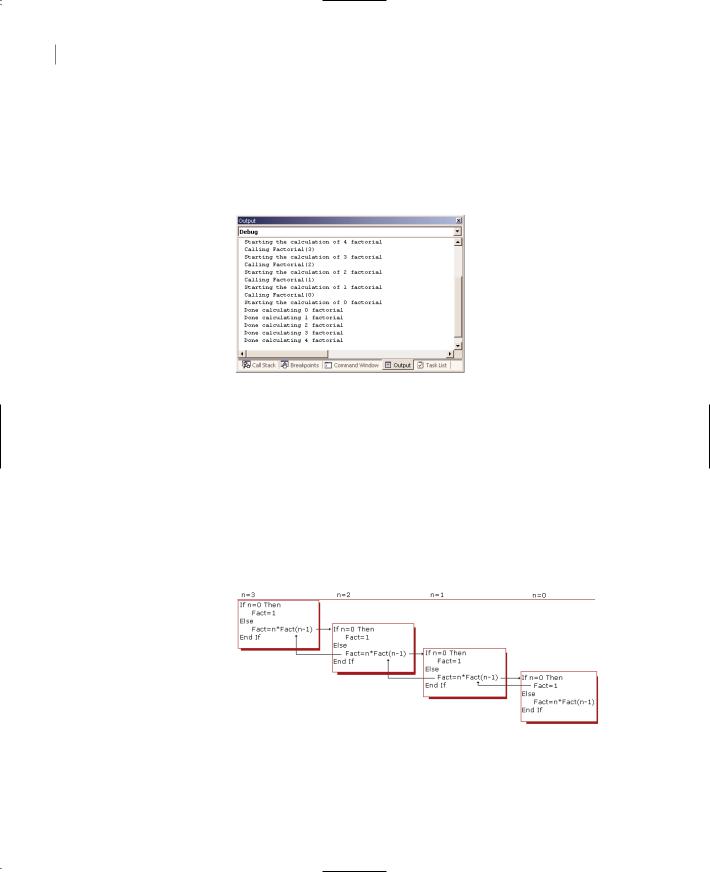
Figure 18.2

You can watch the progress of the calculation of a factorial in the Output window.

When Factorial(0) completes its execution, it prints the following message and returns a result:

Done calculating 0 factorial

This result is passed to the most recently interrupted function, which is Factorial(1). This function can now resume operation, complete the calculation of 1! (1 × 1), and then print another message indicating that it finished its calculations.

As each suspended function resumes operation, it passes a result to the function from which it was called, until the very first instance of the Factorial() function finishes the calculation of the factorial of 4. Figure 18.3 shows this process. (In the figure, factorial is abbreviated as fact.) The arrows pointing to the right show the direction of recursive calls, and the ones pointing to the left show the propagation of the result.

Figure 18.3

Recursive calculation of the factorial of 4

What Happens When a Function Calls Itself

If you’re completely unfamiliar with recursive programming, you’re probably uncomfortable with the idea of a function calling itself. Let’s take a closer look at what happens when a function calls itself.

Copyright ©2002 SYBEX, Inc., Alameda, CA

www.sybex.com

BASIC CONCEPTS 817

As far as the computer is concerned, it doesn’t make any difference whether a function calls itself or another function. When a function calls another function, the calling function suspends execution and waits for the called function to complete its task. The calling function then resumes (usually by taking into account any result returned by the function it called). A recursive function simply calls itself instead of another one.

Let’s look at what happens when the factorial in the previous function is implemented with the following line in which Factorial1() is identical to Factorial():

Factorial = n * Factorial1(n-1)

When the Factorial() function calls Factorial1(), its execution is suspended until Factorial1() returns its result. A new function is loaded into the memory and executed. If the Factorial() function is called with 3, the Factorial1() function calculates the factorial of 2.

Similarly, the code of the Factorial1() function is

Factorial1 = n * Factorial2(n-1)

This time, the function Factorial2() is called to calculate the factorial of 1. The function Factorial2() in turn calls Factorial3(), which calculates the factorial of 0. The Factorial3() function completes its calculations and returns the result 1. This is in turn multiplied by 1 to produce the factorial of 1. This result is returned to the function Factorial1(), which completes the calculation of the factorial of 2 (which is 2 × 1). The value is returned to the Factorial() function, which now completes the calculation of 3 (3 × 2, or 6). As you understand, we can’t write dozens of identical functions; accounting for this is what recursive functions do for your applications.

Recursive Calls and the Operating System

You can think of a recursive function calling itself as the operating system supplying another identical function with a different name; it’s more or less what happens. Each time your program calls a function, the operating system does the following:

1.Saves the status of the active function

2.Loads the new function in memory

3.Starts executing the new function

If the function is recursive—in other words, if the new function is the same as the one currently being executed—nothing changes. The operating system saves the status of the active function somewhere and starts executing it as if it was another function. Of course, there’s no reason to load the code in memory again because the function is already there. The new instance of the function consists of a new set of local variables. The same code will act on different variables and produce a different result. When the newly called function finishes, the operating system reloads the function it interrupted

in memory and continues its execution. I mentioned that the operating system stores the status of a function every time it must interrupt it to load another function in memory. The status information includes the values of its variables and the location where execution was interrupted. In effect, after the operating system loads the status of the interrupted function, the function continues execution as if it was never interrupted. We’ll return to the topic of storing status information later on in the section “The Stack Mechanism.”

Copyright ©2002 SYBEX, Inc., Alameda, CA

www.sybex.com