Matta, Boyd. The quantum theory of atoms in molecules

72 3 Atomic Response Properties

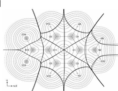
Fig. 3.11 Electron density contours of para-nitroaniline in the nuclear plane, overlaid with interatomic surfaces (bold) and bond paths (semibold).

origin of the molecular coordinate system. For neutral molecules ðQ ¼ 0Þ, m is independent of R0.

As shown in Eq. (1), m can be expressed [2, 3] in terms of atomic dipole polarization contributions, mpðWÞ, and origin-dependent atomic charge-transfer dipole contributions, mcðWÞ:

m ¼	Na		ðW½r R0&rðrÞ dr þ ZW½RW R0&
	X1
	W	¼
¼	Na		ðW½r RW rðrÞ dr þ ½RW R0& ðW rðrÞ dr þ ZW
	X1
	W	¼
	Na		ð
	X

¼½r RW&rðrÞ dr þ ½RW R0&QðWÞ

W¼		1	W
Na						Na
X1			fmpðWÞ þ mcðWÞg ¼			X1				ð14Þ
¼	¼						¼	mðWÞ ¼ mp þ mc
W						W

where QðWÞ is the net charge of atom W. Using Eq. (12), the origin-dependent term mcðWÞ can be expressed in terms of bond charges QðWjLÞ as:

NbðWÞ
X1		ð15Þ
mcðWÞ ¼ ½RW R0&QðWÞ ¼ ½RW R0&	QðWjLÞ

L¼

3.6 Atomic Contributions to Electric Polarizabilities 73

Using Eq. (8), a corresponding origin-independent expression, mcðWÞ, can be defined, as shown in Eq. (5) and below:

NbðWÞ
X1	ð16Þ
mcðWÞ ¼ ½RW RbðWjLÞ&QðWjLÞ

L¼

where RbðWjLÞ is the position vector of the bond critical point between atoms W and L.

Note that for each product RbðWjLÞ QðWjLÞ for atom W, there is a corresponding term for atom L which cancels it, because of Eq. (8), and therefore:

Na

Na

NbðWÞ

X1

X1

X1

mcðWÞ ¼

¼

½RW RbðWjLÞ&QðWjLÞ

W

¼

W

L

¼

Na

Na

X1

X1

mcðWÞ

ð17Þ

¼

¼

RWQðWÞ ¼

¼

W

W

Na

Na

X1

mðWÞ ¼

X1

ðWÞg ¼ mp þ mc

ð18Þ

m ¼

¼

fmpðWÞ þ mc

W

W

¼

Note that all the quantities in the expressions for mpðWÞ and mcðWÞ are uniquely determined by the molecular charge distribution. An essential criterion for any atomic property is that, once formally defined, its evaluation should be uniquely determined entirely by the molecular wavefunction, just as the evaluation of the corresponding molecular property is.

As an example, Table 3.2 shows the z-axis component of mpðWÞ and mcðWÞ and mðWÞ for each symmetrically unique atom in para-nitroaniline (shown in Fig. 3.11), calculated at HF/6-311þþG(2d,2p)//HF/6-311þþG(2d,2p). The total charge-transfer contribution, mc, is over six times that of the opposing total polarization contribution, mp. The dominant contributor to mc is the NO2 nitrogen, N11, especially the contribution from its bond to the ring, mcðN14jC11Þz.

3.6

Atomic Contributions to Electric Polarizabilities

When a molecule is placed in an electric field, its electron distribution changes in response (nuclear geometry changes are assumed to be negligible here). A useful measure of this response is the molecular dipole moment m, whose first derivative and higher derivatives with respect to the electric field correspond to measurable molecular polarizability and hyperpolarizability tensors [13]. Using QTAIM [1], more detailed information about these molecular responses can be obtained, by partitioning the dipole moment and its electric field derivatives into atomic contributions [3, 4].

743 Atomic Response Properties

Table 3.2 Atomic and bond contributions (in a.u.) to the z-axis dipole moment of para-nitroaniline.

Atom, W	m(W)z	mp(W)z	mc(W)z	mc(WSL1)zL1		mc(WSL1)zL2		mc(WSL1)zL3
C1	þ0.381	þ0.751	0.370	0.422 N2		þ0.026 C3		þ0.026 C4
N2	0.010	þ0.170	0.180	0.782 C1		þ0.301 H9		þ0.301 H10
C3	þ0.101	þ0.005	þ0.096	þ0.024 C1		þ0.083	C5	0.011	C6
C5	þ0.144	0.030	þ0.174	þ0.087 C3		þ0.128	C11	0.042	H12
H7	0.072	0.066	0.006	0.006 C3
H10	þ0.016	0.087	þ0.103	þ0.013	N2	þ0.126		þ0.641
C11	þ0.324	0.568	þ0.892	þ0.126	C5		C7		N14
H12	þ0.012	þ0.035	0.023	0.023	C5	þ0.279		þ0.279
N14	þ0.927	0.922	þ1.849	þ1.290	C11		O15		O16
O15	þ0.436	þ0.146	þ0.290	þ0.290 N14
Total[a,b]	þ2.893	0.563	þ3.456

a The analytically calculated value for mðWÞz is þ2.901 a.u.

b An experimental dipole moment for para-nitroaniline (measured in acetone) is 2.44 a.u. [12].

The static dipole polarizability tensor of a molecule, a, is the gradient ð‘EÞ of the molecular electric dipole moment m with respect an external, uniform, and time-independent electric field E, evaluated in the limit of zero field strength:

a ¼ ½‘Em&E¼0 ¼ ½iðqm=qExÞ þ jðqm=qEyÞ þ kðqm=qEzÞ&E¼0	ð19Þ
From Eqs (13) and (19), a is given by:
a ¼ ððr R0ÞrEðrÞ dr	ð20Þ
where the electron density derivative rEðrÞ is given by:
rEðrÞ ¼ ½‘ErðrÞ&E¼0 ¼ ½iðqrðrÞ=qExÞ þ jðqrðrÞ=qEyÞ þ kðqrðrÞ=qEzÞ&E¼0	ð21Þ

Throughout this section, the notation tE is used to indicate the gradient of the term t with respect to E, evaluated at E ¼ 0. In terms of atomic contributions we have, from Section 3.5:

Na		Na		Na
X1		X1		X1
a ¼	¼	aðWÞ ¼	¼	mEðWÞ ¼ fmpEðWÞ þ mcEðWÞg
W		W		W	¼
Na
X1		fapðWÞ þ acðWÞg ¼ ap þ ac				ð22Þ
¼

W¼

3.6 Atomic Contributions to Electric Polarizabilities 75

The atomic dipole polarization gradient with respect to E, apðWÞ ¼ mpEðWÞ, contains a basin (B) contribution, ap; BðWÞ, arising from the density gradient rEðrÞ within the unperturbed atomic basin. It also contains a surface (S) contribution, ap; SðWÞ, arising from the gradient of the atomic surface S with respect to E:

ð

apðWÞ ¼ ðr RWÞrEðrÞ dr þ ap; SðWÞ ¼ ap; BðWÞ þ ap; SðWÞ ð23Þ

W

Similarly, the gradient of the atomic charge transfer dipole contribution with respect to E, acðWÞ ¼ mcEðWÞ, also contains both basin and surface contributions:

acðWÞ ¼ ac; BðWÞ þ ac; SðWÞ			ð24Þ
	NbðWÞ
ac; BðWÞ ¼	X1		ð25Þ
		f½RW RbðWjLÞ&QBEðWjLÞ
	L	¼
	NbðWÞ
ac; SðWÞ ¼	X1		ð26Þ
		½RW RbðWjLÞ&QSEðWjLÞ QðWjLÞRbEðWjLÞ

L¼

Using Eqs (7)–(9), the electric field derivatives of the bond charges, QEðWjLÞ, are determined from the electric field derivatives of the atomic charges QEðWÞ:

ð

QEðWÞ ¼ rEðrÞ dr þ QSEðWÞ ¼ QBEðWÞ þ QSEðWÞ ð27Þ

W

The atomic basin and surface bond charge derivative contributions, QBEðWjLÞ and QSEðWjLÞ, can be obtained separately from the corresponding atomic charge derivatives QBEðWÞ and QSEðWÞ.

The contributions to aðWÞ from the surface derivatives with respect to E arise because both the spatial definition of an atom and an atomic dipole moment contribution are determined entirely by the molecular charge distribution, which is of course dependent on E. This is physically sound (it is physically essential), but it also makes the term-by-term evaluation of apðWÞ and acðWÞ more di cult than usual. However, evaluation of apðWÞ and acðWÞ by numerical di erentiation (using finite field wavefunctions) is straightforward. For example:

apðWÞ k ¼ 1=2f½mpðWÞ&E¼ek ½mpðWÞ&E¼0ge 1
1=2f½mpðWÞ&E¼ ek ½mpðWÞ&E¼0ge 1	ð28Þ

763 Atomic Response Properties

Table 3.3 Atomic contributions (in a.u.) to the principal components of the electric polarizability tensor of para-nitroaniline.

Atom, W	a(W)zz	aB(W)zz	ap(W)zz	ap, B(W)zz	ac(W)zz	ac, B(W)zz
C1	þ9.332	þ10.623	3.152	0.417	þ12.484	þ11.040
N2	þ17.854	þ16.963	0.034	þ5.210	þ17.888	þ11.753
C3	þ12.865	þ13.133	2.792	þ1.458	þ15.657	þ11.674
C5	þ12.077	þ12.220	4.530	þ0.013	þ16.607	þ12.206
H7	þ1.885	þ1.670	þ0.859	þ1.164	þ1.026	þ0.505
H10	þ1.380	þ1.364	þ0.848	þ0.944	þ0.532	þ0.370
C11	þ12.136	þ13.844	0.580	þ1.514	þ12.716	þ12.330
H12	þ1.250	þ1.004	þ0.433	þ0.632	þ0.817	þ0.372
N14	þ16.944	þ15.656	3.830	0.841	þ20.774	þ16.497
O15	þ6.514	þ6.310	þ4.439	þ4.406	þ2.074	þ1.904
Total[a,b]	þ128.214	þ128.487	9.083	þ22.803	þ137.297	þ105.685
Atom, W	a(W)xx	aB(W)xx	ap(W)xx	ap, B(W)xx	ac(W)xx	ac, B(W)xx
C1	þ9.756	þ9.830	4.362	þ0.041	þ14.118	þ9.789
N2	þ4.413	þ4.435	1.590	þ1.799	þ6.002	þ2.637
C3	þ8.125	þ8.385	3.283	þ1.424	þ11.408	þ6.961
C5	þ7.263	þ7.768	3.220	þ1.178	þ10.483	þ6.591
H7	þ3.998	þ3.558	þ0.881	þ1.972	þ3.117	þ1.587
H10	þ1.258	þ1.221	þ0.645	þ0.778	þ0.613	þ0.442
C11	þ9.994	þ9.663	3.354	þ0.637	þ13.348	þ9.026
H12	þ3.260	þ2.936	þ0.845	þ1.673	þ2.415	þ1.263
N14	þ6.975	þ7.367	1.430	0.494	þ8.404	þ7.861
O15	þ7.672	þ7.578	þ2.925	þ3.367	þ4.747	þ4.211
Total[a,b]	þ94.291	þ94.187	13.150	þ22.766	þ107.441	þ71.421

where the average over numerical derivatives for both positive and negative fields is used. Numerical di erentiation to obtain apðWÞ and acðWÞ, together with the straightforward evaluation of the basin contributions (which involve the analytical density derivatives rE) enables the surface derivative contributions to apðWÞ and acðWÞ to be obtained by di erence. Note that the sum of all of the atomic surface derivative contributions is zero:

Na		Na
X1		X1		ð29Þ
aS ¼	¼	aSðWÞ ¼ ½ap; SðWÞ þ ac; SðWÞ& ¼ 0
W		W	¼

			3.6 Atomic Contributions to Electric Polarizabilities					77
Table 3.3	(continued)
Atom, W	a(W)yy	aB(W)yy	ap(W)yy	ap, B(W)yy	ac(W)yy	ac, B(W)yy
C1	þ3.183	þ3.291	þ3.185	þ3.291	0.002	0.000
N2	þ6.950	þ6.936	þ6.983	þ6.936	0.033	0.000
C3	þ6.337	þ6.282	þ6.340	þ6.282	0.003	0.000
C5	þ4.710	þ4.796	þ4.742	þ4.796	0.032	0.000
H7	þ1.115	þ1.113	þ1.117	þ1.113	0.002	0.000
H10	þ0.389	þ0.403	þ0.375	þ0.403	þ0.013	0.000
C11	þ5.136	þ4.853	þ5.113	þ4.853	þ0.023	0.000
H12	þ0.900	þ0.904	þ0.889	þ0.904	þ0.011	0.000
N14	þ2.190	þ2.203	þ2.140	þ2.203	þ0.050	0.000
O15	þ3.497	þ3.586	þ3.504	þ3.586	0.007	0.000
Total[a,b]	þ51.354	þ51.451	þ51.354	þ51.451	0.000

a The analytically calculated values of azz, axx, and ayy are þ128.487, þ94.187, and þ51.451 a.u.

b The experimentally measured isotropic polarizability (measured in acetone) is þ114.73 a.u. [12] compared with the analytically calculated isotropic value of þ91.375 a.u.

Thus, the molecular polarizability a can be written as:

Na		Na
X1		X1
a ¼	¼	aðWÞ ¼ ½apðWÞ þ acðWÞ&
W		W	¼
Na
X1		½ap; BðWÞ þ ac; BðWÞ þ ap; SðWÞ þ ac; SðWÞ& ¼ aB þ aS ¼ aB		ð30Þ
¼

W¼

That the sum of the atomic surface derivative contributions vanishes does not necessarily mean they should be ignored, however, especially when comparing and/or transferring atomic polarizabilities between molecules.

Using the partitioning method outlined above, Bader et al. [4] studied, among other things, the atomic and group contributions to the polarizability tensors of the normal alkane series and showed that the empirical additivity relationship for the isotropic polarizability of normal alkanes in terms of transferable methylene and methyl group contributions is mirrored by the corresponding theoretical group contributions, thus providing a theoretical basis for the empirical relationship or an experimental validation for the theoretical definition of QTAIM polarizabilities.

As an example here, Table 3.3 shows the diagonal components of apðWÞ and acðWÞ and aðWÞ for each symmetrically unique atom of para-nitroaniline, calculated using the coupled–perturbed HF/6-311þþG(2d,2p)//HF/6-311þþG(2d,2p) level of theory. Also shown in Table 3.3 are the corresponding basin contributions

78 3 Atomic Response Properties

Fig. 3.12 E ect of a finite (0.05 a.u.) electric field applied along the z-axis of para-nitroaniline in terms of electron density contours, interatomic surfaces (bold), and bond paths (semi-bold) in the nuclear plane. Dotted lines correspond to the presence of the field whereas solid lines correspond to the absence of the field.

ap; BðWÞ, ac; BðWÞ, and aBðWÞ. The magnitude of the total charge-transfer contribution to azz is over fourteen times that of the opposing total polarization contribution. The polarizability axx is similarly dominated by charge transfer whereas the much smaller ayy is due entirely to atomic polarization, the charge-transfer contribution vanishing by symmetry (the non-zero values shown for acðWÞyy provide a measure of the error in the results for the other atomic polarizability contributions). That the sum of aðWÞzz does not equal the sum of aBðWÞzz ¼ azz is because of error in the numerical di erentiation used to obtain the total (basin þ surface) aðWÞzz contributions, whereas the aBðWÞzz contributions were calculated from the analytical density derivative. Similar statements apply for the yy and zz components. Figure 3.12 shows the e ect on the charge distribution of a finite external electric field (0.05 a.u.) applied along the z-axis. Note that the shift in electronic charge is opposed to the electric field whereas the shift in the interatomic surfaces is in the opposite direction [3].

3.7

Atomic Contributions to Vibrational Infrared Absorption Intensities

Within the (double) harmonic approximation, the intensity of absorption, I, of a peak in an infrared spectrum for a molecule is proportional to the first derivative

3.7 Atomic Contributions to Vibrational Infrared Absorption Intensities 79

of the electric dipole moment, m, of the molecule with respect to one of the normal-mode vibrational coordinates x (a combination of nuclear displacement coordinates from an equilibrium geometry), in the limit of x ¼ 0. For a normal mode of vibration with frequency nx and normal coordinate x, the corresponding theoretical absorption intensity, Ix, is [13, 14]:

Ix ¼ Cjðdm=dxÞx¼0j2 ¼ Cjmxj2

ð31Þ

where C is a collection of constants and the notation tx is used to indicate the derivative of the term t with respect x, evaluated at x ¼ 0. Absorption intensities of vibrational spectra can be understood in terms of atomic and bond contributions using the equations in Section 3.5 with Eq. (31). The formalism is similar to that for polarizabilities:

Na		Na
X1		X1		ð32Þ
mx ¼	¼	mxðWÞ ¼ fmpxðWÞ þ mcxðWÞg ¼ mpx þ mcx
W		W	¼
mpxðWÞ ¼ ðWðr RWÞrxðrÞ dr þ RWxQðWÞ þ mp; SxðWÞ
	¼ mp; BxðWÞ þ mp; SxðWÞ			ð33Þ

NbðWÞ

X

mcxðWÞ ¼ f½RW RbðWjLÞ&Q xðWjLÞ þ RWxQðWjLÞ QðWjLÞRbxðWjLÞg

L¼1

NbðWÞ

X

¼f½RW RbðWjLÞ&QBxðWjLÞ þ RWxQðWjLÞg

L¼1

			þ	NbðWÞ
				X f½RW RbðWjLÞ&QSxðWjLÞ QðWjLÞRbxðWjLÞg
				L¼1
	¼ mc; BxðWÞ þ mc; SxðWÞ						ð34Þ
	Na				Na
X1					X1		ð35Þ
mSx ¼		¼	mSxðWÞ ¼			½mp; SxðWÞ þ mc; SxðWÞ& ¼ 0
W					W	¼
Na				Na
X1				X1
mx ¼	¼		mxðWÞ ¼		¼	½mpxðWÞ þ mcxðWÞ&
W				W

Na

X

¼½mp; BxðWÞ þ mc; BxðWÞ þ mp; SxðWÞ þ mc; SxðWÞ&

W¼1
¼ mBx þ mSx ¼ mBx	ð36Þ

80 3 Atomic Response Properties

The normal coordinate derivatives of the bond charges QxðWjLÞ and their basin and surface contributions, QBxðWjLÞ and QSxðWjLÞ, are determined from the corresponding atomic charge derivatives QxðWÞ using Eqs (7)–(9). QxðWÞ is given by:

ð

QxðWÞ ¼ rxðrÞ dr þ QSxðWÞ ¼ QBxðWÞ þ QSxðWÞ ð37Þ

W

When compared with the corresponding polarizability term apðWÞ, the term mpxðWÞ contains an additional contribution RWxQðWÞ, which is the atomic charge-weighted derivative of the nuclear position RW with respect to xk. Similarly, the charge-transfer term mcxðWÞ contains an extra contribution for each bond, RWxQðWjLÞ, which is the bond-charge-weighted derivative of the nuclear position RW with respect to coordinate x.

Like the atomic polarizability contributions, the term-by-term evaluation of the atomic polarization and charge-transfer contributions to an electric dipole derivative with respect to a normal vibrational coordinate is complicated (but in a physically necessary way) by the dependence of the atomic surfaces on the nuclear positions. As with the polarizabilities, however, the total mpxðWÞ and mcxðWÞ can each be easily evaluated by numerical di erentiation and the terms involving the analytical density derivative rxðrÞ can be evaluated directly, thus enabling the surface derivative contributions to be obtained by di erence.

Bader et al. [2] were the first to study molecular dipole moment changes associated with normal mode vibrations using QTAIM. Their analysis used finite displacements along a normal coordinate or symmetry coordinate to observe changes in mpðWÞ and an origin-dependent charge-transfer contribution which is somewhat di erent, and less generally applicable, than the mcðWÞ given here, but their results clearly showed that changes in atomic polarizations, changes in atomic charges, and displacement of atomic charges are all important in understanding dipole moment derivatives with respect to normal mode vibrational coordinates, and hence IR spectra.

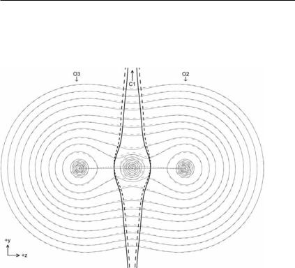
As an example here, Table 3.4 shows the atomic contributions mxðWÞ, mpxðWÞ, and mcxðWÞ to the molecular dipole derivative mx for one of the pair of degenerate bending normal modes of vibration in CO2 and the asymmetric stretching normal mode, calculated at the coupled–perturbed HF/6-311þþG(2d,2p)//HF/6- 311þþG(2d,2p) level of theory. For the bending mode, shown in Fig. 3.13, the calculated dipole derivative is þ0.879 a.u. directed along the y-axis. For the asymmetric stretch, shown in Fig. 3.14, the calculated dipole derivative is 3.793 a.u. directed along the z-axis. The di erence between the calculated dipole derivatives is in good agreement with experimental results [15]. For the bending mode, the atomic polarization derivatives are counter to the larger magnitude atomic charge-transfer derivatives. In contrast, for the asymmetric stretching mode, both the atomic polarization derivatives and the atomic charge transfer derivatives contribute positively to the overall dipole derivative, making it much larger.

3.7

Atomic Contributions to Vibrational Infrared Absorption Intensities

81

Table 3.4

Atomic contributions to the dipole moment derivatives of CO2

(in a.u.) with respect to the bend and asymmetric stretch (AS) normal

mode coordinates. Also shown are the atomic charge Q derivatives.[a,b,c]

Atom, W

mBend(W)

y

m

Bend(W)

y

m Bend(W)

y

QBend(W)

p

c

C1

þ0.191

0.741

þ0.932

0.012

O2

þ0.342

0.795

þ1.137

þ0.006

O3

þ0.342

0.795

þ1.137

þ0.006

Total

þ0.876

2.331

þ3.207

þ0.000

Atom, W

mAS(W)

m

AS(W)

z

m

AS(W)

z

QAS(W)

z

p

c

C1

þ1.655

þ1.213

þ0.442

0.049

O2

þ1.068

þ0.780

þ0.288

0.508

O3

þ1.055

þ0.898

þ0.157

þ0.573

Total

þ3.778

þ2.891

þ0.887

þ0.016

a Calculated frequencies for the modes are 776 (bend) and 2551 (AS) cm 1.

b Experimental frequencies for the modes are 667 (bend) and 2349 (AS) cm 1. c The experimentally measured ratio of the AS and bend dipole derivatives

is 4.57 [15], compared to the calculated ratio of 4.31.

Fig. 3.13 E ect of finite ðx A0:2 a.u.) bending vibration on CO2 in terms of electron density contours, interatomic surfaces (bold), and bond paths (semi-bold). Dotted lines correspond to bent geometry whereas solid lines correspond to equilibrium geometry.