Matta, Boyd. The quantum theory of atoms in molecules

122 5 Topological Atom–Atom Partitioning of Molecular Exchange Energy

a change in nuclear positions. This method deals with polarization and is currently under investigation in our laboratory.

Although the literature on the application of point-charge potentials is huge, it is recognized they have inherent limitations, for example the modeling of lone pairs and aromatic rings. Several groups (including one in Accelrys) have noticed the limitations of point charges in their work and make explicit statements [7–18] in support of multipoles. For example, in their work on the prediction of (crystal) polymorphs Day et al. [11] went as far as to assert, that ‘‘the atomic charge calculations might have motivated an exploration of kinetic reasons why hydrogen bonded dimers are found in the crystal structure of oxazolidine-2,5-dione in preference to chains; energy calculations with the atomic multipoles model suggest that the preference is simply energetic and any exploration of other determining factors would have been illfounded.’’ Another important example is that of Batista et al. [19], who stated that ‘‘point-charge models are typically tailored to be consistent with various properties of liquid water, but may not reproduce accurately the electric fields in other environments, such as water clusters, ice, surfaces, and interfaces.’’ This insight is important for peptide solvation and docking, where small interstitial water clusters can appear.

Over the last few years we have systematically explored the behavior of multipole moments of topological atoms. In a study on the atomic partitioning of the molecular potential [20] we demonstrated the favorable convergence of the topological multipole expansion and the reason why [21]. Via a continuous multipole method involving Bessel functions it was subsequently proven [22] that the region of convergence of the potential could be enlarged. The introduction of inverse moments [23] enabled the potential to converge everywhere. The electrostatic interaction between topological atoms could also be successfully expressed as a convergent multipole expansion and could therefore be used for prediction [24] of van der Waals complexes and hydrogen-bonded DNA base pairs [25]. The convergence of the multipole expansion received attention [26] in atom–atom partitioning of intramolecular and intermolecular Coulomb energy. In that work seven systems were analyzed – an ethyne dimer, a hydrogen fluoride dimer, a water dimer, butane, 1,3,5-hexatriene, acrolein, and cis-urocanic acid. The current work can be seen as a counterpart of that study but for the exchange interaction rather than the Coulomb interaction. Here we focus on the same systems except the last. Here, however, the convergence analysis is extended to higher rank and includes forces rather than just energies.

As far as we know there is no force field that incorporates exchange energy, but it is possible that it will feature in a future force field. Similarly, the kinetic energy, another term in the energy partitioning of any quantum system [27], does not feature in force fields. Yet, these terms greatly a ect the total energy surface of molecules and molecular assemblies and hence their structure and dynamics. Their e ect is typically absorbed in the fitted bonded and non-bonded terms. In this contribution we only touch upon the question of how exchange energy may be adopted by a force field. As before, aware of the complexity of this question, we judge it to be important to first systematically analyze the convergence behavior of a high-rank multipole expansion of the exchange energy. That such an analysis

5.2 Theoretical Background 123

can lead to unexpected results was proven in a recent paper [28], which showed that both 1,3 and 1,4 interactions can be described on the same footing as 1,n ðn > 4Þ interactions by a convergent multipole expansion of the Coulomb energy of the participating atom pairs.

5.2

Theoretical Background

Within the Born–Oppenheimer approximation the total closed-shell Hartree– Fock energy is given by:

E ¼ 2

ð dr1

‘1 rðr1; r2Þjr1 ¼r2

þ

2 ðð dr1 dr2

rtot

ð

rÞ12

ð

r2

Þ

1

2

1

r1 rtot

ðð dr1 dr2

ð

2rÞ121

ð

1Þ

4

1

r

1

; r

r

2

; r

ð1Þ

1

r

r

where rtot is the total charge density, r12 is the inter-electron distance, and r1ðr1; r2Þ the first-order reduced density matrix or one-matrix. The latter is given by:

r1ðr1; r2Þ ¼ 2 Xci ðr1Þciðr2Þ ð2Þ

i

where the sum runs over molecular orbitals ci. The diagonal of this density matrix is the electron density, rðrÞ, which combined with the (total) nuclear charge density yields the total charge density:

rtotðrÞ ¼	X	ð3Þ
	ZAdðr RAÞ rðrÞ
	A
The first term in Eq. (1) defines the kinetic energy and jr1 ¼r2		means the coordi-

nates r1 and r2 are kept separated until the Laplacian has operated on only one c, whereupon the coordinates are set equal to each other.

The total energy can be partitioned in terms of topological atoms, denoted W, via:

E ¼ 2

ð

dr1‘21rðr1; r2Þjr1¼r2

þ 2

ð

dr1

ð

dr2

totð

1rÞ12totð

2Þ

1

X

1

XX

r

r

r

r

A

WA

A

B

WA

WB

4

ðWA dr1 ðWB dr2

1ðr1

ð4Þ

r

;

r2rÞ121ðr2

;

r1Þ

1

XX

r

A

B

124 5 Topological Atom–Atom Partitioning of Molecular Exchange Energy

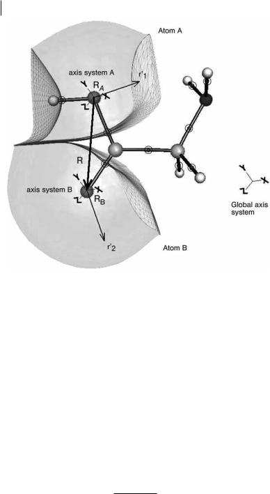
Fig. 5.1 Atomic basins of the oxygen atoms in glycine. The nuclei are shown as spheres. The bond critical points are shown by encircled dots. The interatomic surfaces are represented by small triangles. The basins are capped by an isodensity envelope at 10 3 au. R represents the internuclear vector, RA

and RB the positions of the nuclei A and B in the global axis system, and r1 and r2 describe the electron density in the basins A and B, respectively. The global axis system is shown outside the molecule and centered on the global origin.

where the double sum			A	ð		B is not restricted in any way, i.e. the interaction
between two di erent	atoms				A		0	B	is counted twice and the self-interaction of
		P	P

each atom ðA ¼ BÞ is included. The second group of terms expresses the Coulomb interaction and featured in earlier work [26]. This work focuses on the third group of terms. Figure 5.1 clarifies how the inter-electron distance r12 is related to the internuclear distance and the nuclear positions.

Because the molecular orbitals are real it follows that r1ðr1; r2Þ ¼ r1ðr2; r1Þ and, because r12 ¼ jR þ r2 r1j, the exchange energy between atoms A and B (appearing in Eq. 4) has the form:

X

¼ ð

1 ð

2

Rj

ð r

r

2

ð

Þ

E AB

dr

dr

r1

r1

; r2Þj

5

j

þ

1j

WA

WB

2

5.2 Theoretical Background 125

Computation of the exchange energy in Eq. (5) involves a six-dimensional (6D) integral. The same type of integral has to be evaluated in the computation of the Coulomb interaction but there the numerator, rtotðr1Þrtotðr2Þ, is already separated (or factorized) in terms of the variables r1 and r2. Because of the entanglement between variables r1 and r2 in the one-density matrix, the 6D integration for the exchange energy is much slower than its Coulomb counterpart. Indeed, if there are n quadrature points in each atomic grid, the numerator (i.e. the one-electron density matrix) must be evaluated for each pair of grid points, or n2 times. In the Coulomb 6D integral, on the other hand, the charge density of each basin must be evaluated in n quadrature points, corresponding to only 2n evaluations of the electron density in total. In practice, the most straightforward way of separating the variables r1 and r2 is to express r1ðr1; r2Þ by means of molecular orbitals:

EXAB ¼ 4 ð

dr1 ð

dr2

ð

ÞR ð

rÞ

ð r Þ

ð

Þ

ð6Þ

Xi

Xj

ci

r1

ci

r2

cj r1

cj

r2

WA

WB

j þ 2 1j

where i and j are summed throughout the molecular orbitals. At this stage it is convenient to define the overlap function at a point r:

SijðrÞ ¼ 2ciðrÞcjðrÞ

ð7Þ

where we point out that the occupation number of two is absorbed in Sij. Substituting Eq. (7) into Eq. (6) leads to:

EX	¼ ð	dr1 ð	dr2			R r	r Þ	ð8Þ
AB				Xi	Xj	Sijðr1ÞSijðr2
	WA		WB			j þ 2 1j

This 6D integral is computationally less expensive to evaluate than that in Eq. (5), because the overlap function is computed in the two atomic grids separately,

which is reminiscent of the computation of rtotðr1Þrtotðr2Þ. The cost of Eq. (8) is still larger than the 6D integration of the Coulomb energy, however.

Both the exchange and Coulomb energy can be expressed via a multipole expansion, which has been described in detail before [26]. At the cost of possible lack of convergence this expansion separates the variables R, r1, and r2, which are entangled in the expression jR þ r2 r1j 1.

A binomial Taylor expansion of jR þ r2 r1j 1 and subsequent application of an addition theorem for regular spherical harmonics [29, 30] factorizes the electronic ðr1; r2Þ and geometric (R) coordinates as follows:

1

y

y

l1

l2

¼ lX1 0 lX2 0 mX1

mX2

l2 Tl1 l2 m1m2 ðRÞRl1m1 ðr1ÞRl2m2 ðr2Þ

ð9Þ

l1

j

R

þ

r2

r1

j

¼

¼

¼

¼

126 5 Topological Atom–Atom Partitioning of Molecular Exchange Energy

and

	l1l2m1m2						sð
T		ð	R		1	l1	2l1 þ 2l2 þ 1Þ!
				Þ ¼ ð Þ			ð2l1Þ!ð2l2Þ!		!Il1þl2; ðm1 þm2ÞðRÞ
						l1	l2	l1 þ l2		ð10Þ
						m1 m2		ðm1 þ m2Þ

where the expression in large brackets is a Wigner 3j symbol and RlmðrÞ and IlmðrÞ are the regular and irregular normalized spherical harmonics Ylmðy; jÞ, respectively:

Rlm

r

rr lYlm

y; j

11a

ð Þ ¼

4p

ð

Þ

ð

Þ

2l

þ

1

Ilm

r

rr l 1Ylm

y; j

11b

ð Þ ¼

4p

ð

Þ

ð

Þ

2l

þ

1

The terms in Eq. (9) can be conveniently grouped according to the power of the interaction distance RAB ðl1þl2þ1Þ ¼ RAB L by use of Eq. (11b), where L monitors the rank of the expansion.

Substituting Eq. (9) into Eq. (8) leads to:

EX	y	y	l1	l1	l2	Tl1 m1 l2m2 ðRÞ Xij	Ql1 m1	ðWAÞQl2m2 ðWBÞ	ð12Þ
	¼ lX1 0 lX2 0 mX1				mX2 l2
AB							ij	ij
	¼	¼	¼		¼

where the exchange moments, QijlmðWÞ, unlike their Coulomb counterpart (the familiar atomic multipole moments), explicitly depend on the molecular orbitals:

ð

QijlmðWÞ ¼ drSijðrÞRlmðrÞ ð13Þ

W

Note that both the overlap function Sij (Eq. 7) and the electron density (deduce from Eq. 2) incorporate the occupation number. Because they share this feature with (atomic) electrostatic multipole moments, defined as Q lmðWÞ ¼

W drrðrÞRlmðrÞ, they have a very close and simple relationship with exchange mo-
Ðments, i.e. Q lmðWÞ ¼		i QiilmðWÞ.
For completeness	we point out that Eq. (10) is only valid when all multipole
		P

moments are expressed relative to the global axis system. It is possible to work with moments that are expressed relative to their own local atomic axis system. In this more general approach each atomic frame can take on an arbitrary orientation. For mathematical details we refer to Section 3.3 in Stone’s book [30]. In our current analysis, however, there is no need for this generalization, because we analyze single molecules and supermolecules, each expressed relative to a sin-

5.2 Theoretical Background 127

gle global axis system. Each atomic local frame has the same orientation as the global frame, and this is just a special case of the more general approach described above. We mention the general approach, however, because it is in this context that Ha¨ttig [31] developed his recurrence formula for computation of the interaction tensor TðRÞ. This formula enables evaluation of this tensor to an arbitrarily high rank L. Hence we can now go beyond the limitation of L ¼ 5 of previous work, where explicit (i.e. pre-calculated) formulae for TðRÞ were used. The evaluation of explicit formulae, as listed up to rank L ¼ 6 [30, 32], is more rapid, however.

The exact exchange force is defined by Eq. (14).

FXAB ¼ 4 ð

dr1 ð

dr2

ð

Þ

ð

rÞ3

ð

Þ

ð

Þ r12

ð14Þ

ci

r1

ci

r2

cj

r1

cj

r2

WA

WB

Xi

Xj

12

It is straightforward to di erentiate Eq. (12) to obtain the kth force component from the exchange energy:

y	y	l1	l2	qRA; k	ð	R	Þ Xij		Ql1 m1	ðWAÞQl2m2 ðWBÞ	ð15Þ
FX; k ¼ lX1 0 lX2 0 mX1			l1 mX2 l2
AB				qTl1m1 l2 m2					ij	ij
¼	¼	¼	¼

where RA; k is the kth component of the position vector of the nucleus A and where we have assumed that the exchange moments do not vary with a change in nuclear positions. Note that Ha¨ttig’s recursive formulae are easy to di erentiate with respect to nuclear components.

The development so far has focused on (closed-shell) Hartree–Fock wave functions, but it is possible to extend the multipole formalism to post Hartree–Fock wave functions. The total (electronic) interaction energy between two topological atoms is given by Eq. (16):

ee	¼ ð		1 ð		2		R r		r		ð Þ
E AB		dr		dr			r2ðr1	; r2	Þ		16
						j	þ 2			1j
	WA		WB

where the second-order reduced density matrix r2ðr1; r2Þ can be written in terms of molecular orbitals as follows:

X	ð17Þ
r2ðr1; r2Þ ¼ Cijklciðr1Þcjðr1Þckðr2Þclðr2Þ

ijkl

The only nonvanishing C coe cients at the Hartree–Fock level are Ciijj ¼ 2 and Cijji ¼ 1. Equation (6) is reproduced by inserting Eq. (17) into Eq. (16) and collecting the terms in the quadruple sum of Eq. (17) corresponding to Cijji ¼ 1. The multipole expansion for post-Hartree–Fock wave functions is generalized in a straightforward manner in Eq. (18).

128 5 Topological Atom–Atom Partitioning of Molecular Exchange Energy

	y	y	l1	l2	X
AB	lX1 0 lX2 0 mX1			l1 mX2 l2		ij		kl
Eee	¼	¼	¼	Tl1m1l2m2 ðRÞ		CijklQl1 m1	ðWA	ÞQl2m2	ðWBÞ	ð18Þ
	¼			¼	ijkl
We note	that	Pendas		et al. [33]	developed	a monadic		diagonalization of

r2ðr1; r2Þ to avoid the computational overhead because of the extra four summations occurring in Eqs (17) and (18). Using CI wave functions Fradera et al. [34] and Poater et al. [35] calculated electron localization and delocalization indices for topological atoms. Their indices are functions of SijðWÞ, which can be identified

with a ‘‘monopolar exchange moment’’ ðl ¼ m ¼ 0Þ, because from Eq. (13) we learn that QijooðWÞ ¼ ÐW drSijðrÞ, because R00ðrÞ ¼ 1. In their work the Cijkl coe - cients were extracted from the ab initio code GAMESS, an involved procedure

that was avoided by Wang and Werstiuk [36]. Taking advantage of the so called Z-vector method [37] they developed a simpler way to include the Coulomb correlation e ects. By introducing natural molecular orbitals and non-integer occupation numbers the equations developed at the Hartree–Fock level can be retained for post-Hartree–Fock wave functions.

Because, in this study, we used B3LYP wave functions we need to comment on the validity and re-interpretation of the multipole formalism, especially Eq. (12) and some equations leading up to it. There are inherent di erences between the exchange-correlation of the Kohn–Sham formalism and Hartree–Fock formalism [38, 39]. With Kohn–Sham density-functional theory the total electronic energy of the real, fully-interacting system is expressed as:

Etot ¼ T0	þ	ð drrVnuc þ 2	ðð dr1 dr2	ð	1rÞ12ð	2Þ	þ EXC	ð19Þ
		1		r r	r r

where T0 is the kinetic energy of the non-interacting reference system, and the second and third terms are the nuclear interaction energy and the Coulomb energy, respectively. The last term, EXC, actually defines the Kohn–Sham exchangecorrelation energy. It contains, buried within it, all the details of two-body exchange and a kinetic-energy component. Inserting Kohn–Sham orbitals in Eq.

(8) to compute and analyze what looks like an ‘‘exchange’’ energy can be justified on the grounds of the generality of r1ðr1; r2Þ in Eq. (5) and the similarity between the Kohn–Sham scheme and the Hartree–Fock scheme. The essence of this work is to investigate the convergence of multipole expansions of a substantial contribution to the total energy, which is not the Coulomb energy or the exact kinetic energy. For easy reference we will refer to this energy contribution simply as the ‘‘exchange energy’’.

5.3

Details of Calculations

We have modified the program MORPHY01 to integrate the exchange moments Qijlm for a pair of molecular orbitals ði; jÞ. The moments are written in an output

5.3 Details of Calculations 129

file. The CPU time required for the integration limited the maximum rank of the moments computed to L ¼ 10. The atomic basins are capped at the r ¼ 10 7 a.u. isodensity envelope. Because these calculations are computationally demanding we used the default grid of MORPHY01 for the 3D integration of the moments, the number of radial and angular quadrature points being set at ðnr; ny; njÞ ¼ ð80; 30; 50Þ for the b sphere and ð70; 50; 80Þ for the rest of the atomic basin. The interaction tensor TðRÞ, and its derivatives, were calculated up to an arbitrary rank L by use of an in-house program containing Ha¨ttig’s recurrence formulae. MORPHY01 was previously used [26] to obtain the (‘‘exact’’, i.e. non-expanded) Coulomb energy between two topological atoms. This program was modified to compute the exact exchange energy and force for two topological atoms by 6D numerical integration.

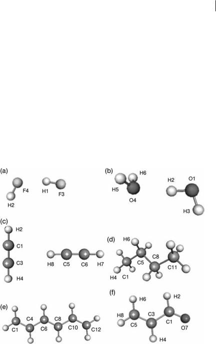
Figure 5.2 shows the geometry and numbering scheme of the six systems studied. All molecules were optimized, without imposed symmetry, by the program GAUSSIAN03 [40] at the same of level of theory, B3LYP/6-311 þ G(2d,p), as in the earlier counterpart study [26] on the Coulomb interaction.

Fig. 5.2 Geometry and numbering scheme of the six systems studied:

(a) HF dimer, (b) H2O dimer, (c) C2H2 dimer, (d) butane, (e) 1,3,5- hexatriene, (f ) acrolein.

atom–atom interactions (

¼ 6). It is clear that the multipole expansion does

1305 Topological Atom–Atom Partitioning of Molecular Exchange Energy

Table 5.1 Exchange energy (kJ mol 1) between atomic basins with increasing nuclear separation R in (HF)2 from multipole expansion (increasing rank L) and 6D numerical integration (exact).

	H1xF3[a]	H2xF4[a]	H1xF4	H1xH2	F3xF4	H2xF3
R (a.u.)	1.76	1.75	3.44	4.49	5.17	6.02
L ¼ 1	660.7	733.0	44.0	0.4	35.6	0.4
L ¼ 2	723.6	747.9	61.3	0.4	46.9	0.3
L ¼ 3	791.1	858.6	68.0	0.4	51.1	0.3
L ¼ 4	784.2	822.1	70.1	0.4	52.1	0.3
L ¼ 5	702.0	725.7	70.2	0.4	52.5	0.3
L ¼ 6	694.0	773.7	69.5	0.4	52.7	0.3
L ¼ 7	770.3	742.1	68.9	0.4	52.7	0.3
L ¼ 8	759.4	699.4	68.8	0.4	52.5	0.3
L ¼ 9	672.4	1272.6	69.1	0.4	52.2	0.3
L ¼ 10	823.4	791.2	69.6	0.4	52.2	0.3
Exact	740.4	783.6	69.8	0.4	52.4	0.3

a Note that in this and subsequent tables the bonded interactions (i.e. between two atoms separated by one or two bonds, or 1,2 and 1,3 interactions) are colored in light grey.

5.4

Results and Discussion

5.4.1

Convergence of the Exchange Energy

The HF dimer often appears as a simple prototype system featuring medium to

strong hydrogen bonding between polar molecules. Table 5.1 shows all possible

4

2

not converge for the nearly equivalent covalently bonded atoms (H1–F3 and H2– F4), as is observed for the corresponding Coulomb interaction. It is pleasing to learn that the hydrogen bonded interaction (H1–F4) stabilizes rapidly toward the exact value of 69.8 kJ mol 1, already at L ¼ 4. This was also observed for the hydrogen bond Coulomb interaction. Perhaps surprising is the rather sizeable (but properly converged) exchange energy between the fluorine atoms.

The exact and multipole expanded exchange energies of eleven relevant interactions in the water dimer are presented in Table 5.2. There is a total of 62 ¼ 15

interactions but four can be left out because of (near) planar symmetry. The pattern observed here is very similar to that of the HF dimer. As expected, the multipole expansion is unable to converge for bonded interactions. For the non-bonded

5.4 Results and Discussion 131

Table 5.2 Exchange energy (kJ mol 1) between atomic basins with increasing nuclear separation R in (H2O)2 from multipole expansion (increasing rank L) and 6D numerical integration (exact). The labels correspond to those in Fig. 5.2.

	O4xH5	O1xH3	O1xH2	H2xH3	H5xH6	H2xO4	H2xH5
R (a.u.)	1.82	1.82	1.84	2.90	2.90	3.66	4.62
L ¼ 1	1009.0	1064.8	870.8	7.5	8.4	55.3	0.7
L ¼ 2	1087.6	1135.9	1002.5	4.9	5.1	78.6	0.7
L ¼ 3	1214.7	1269.6	1080.4	5.8	6.5	87.6	0.6
L ¼ 4	1170.3	1232.6	1062.6	5.6	6.0	90.1	0.6
L ¼ 5	994.6	1021.9	940.2	5.5	6.1	89.6	0.6
L ¼ 6	1060.3	1098.5	905.2	5.6	6.2	88.3	0.6
L ¼ 7	1151.3	1274.7	1072.9	5.6	6.1	87.4	0.6
L ¼ 8	944.3	917.7	1170.6	5.6	6.1	87.6	0.6
L ¼ 9	2009.2	2171.8	763.8	5.6	6.1	88.4	0.6
L ¼ 10	1565.1	2265.0	702.7	5.7	6.2	88.9	0.6
Exact	1109.6	1161.1	1003.7	5.6	6.1	88.2	0.7

	O1xO4	O1xH5	H3xO4	H3xH5
R (a.u.)	5.49	6.31	6.34	7.38
L ¼ 1	34.6	0.5	0.8	0.0
L ¼ 2	44.8	0.5	0.8	0.0
L ¼ 3	48.4	0.5	0.8	0.0
L ¼ 4	48.8	0.5	0.8	0.0
L ¼ 5	49.1	0.5	0.8	0.0
L ¼ 6	49.3	0.5	0.8	0.0
L ¼ 7	49.3	0.5	0.8	0.0
L ¼ 8	49.0	0.5	0.8	0.0
L ¼ 9	48.8	0.5	0.8	0.0
L ¼ 10	48.8	0.5	0.8	0.0
Exact	49.0	0.5	0.8	0.0

interactions, however, the expansions predict a value very close to that from 6D integration. Even at short range (for instance the H2–H3 and H5–H6 interactions), for which the Coulomb expansion is expected to fail, the exchange interaction has an error of less than 0.1 kJ mol 1. There are only small di erences (less than 1 kJ mol 1) between the expansions at rank L ¼ 6 and L ¼ 10 for nonbonded interactions. Although the bonded OaH interaction largely dominates the other interactions, the intermolecular interactions between H2 and O4, which represents the hydrogen bond, and the oxygen–oxygen interactions are not negli-