Matta, Boyd. The quantum theory of atoms in molecules

Table 1.1 Comparison of the molecular dipole moments of some amino acids obtained from group contributions with those obtained directly from SCF calculations.[a,b] The table also compares the second letter of the genetic code of each amino acid with side-chain dipole. (Adapted from Refs. [56, 60]).

Amino	Second	Nature
acid	base in	of the 2nd
	the mRNA	base[d] in
	genetic	the codon
	codon[c]

Side-chain dipole[a,b] (au)

Main-chain dipole[a,b] (au)

Total molecular dipole[a,b] (au)

Rx

xCH(NH2)COOH

RxCH(NH2)COOH

mx

my

mz

|m|

mx

my

mz

|m|

mx

my

mz

|m|

Gly	G	I	0.006	0.068	0.098	0.119	0.415	0.376	0.095	0.568	0.409	0.307	0.002	0.512
					0.074		0.363		0.267		0.402	0.317 0.001 0.512
Ile	U	II	0.130	0.012		0.150		0.521		0.689	0.233	0.533	0.341	0.674
				0.108	0.120				0.073		0.207	0.537	0.269	0.635
Ala	C	II	0.034			0.165	0.217	0.590		0.632	0.251	0.481	0.193	0.576
			0.103		0.062			0.621	0.266		0.252	0.480	0.193	0.576
Val	U	II		0.149		0.191	0.097			0.683	0.006	0.473	0.328	0.575
							0.195	0.607			0.013	0.473	0.319	0.571
Leu	U	II	0.069	0.182	0.081	0.211			0.163	0.658	0.127	0.424	0.244	0.506
				0.142	0.118		0.099		0.057		0.119	0.412	0.264	0.503
Phe	U	II	0.217			0.285		0.642		0.652	0.118	0.501	0.175	0.543
			0.292	0.401	0.201			0.622	0.065		0.077	0.495	0.187	0.535
Tyr	A	I				0.536	0.138			0.641	0.154	1.024	0.266	1.069
				0.259	0.548			0.645			0.137	1.026	0.272	1.071
Thr	C	II	0.399			0.726	0.114		0.065	0.658	0.514	0.904	0.483	1.147
			0.377	0.636	0.327		0.288	0.005	0.382		0.515	0.904	0.479	1.146
Met	U	II				0.809				0.479	0.665	0.642	0.709	1.165
											0.661	0.647	0.695	1.157

Molecules in Atoms of Theory Quantum the to Introduction An 1 22

Trp	G	I	0.354	0.727	0.140	0.820	0.084	0.498	0.173	0.534	0.270	1.225	0.313	1.293
			0.692				0.366		0.479		0.245	1.233	0.315	1.296
Cys	G	I		0.090	0.450	0.830		0.017		0.603	1.058	0.107	0.029	1.064
			0.823	0.091				0.428	0.047		1.047	0.118	0.033	1.055
Ser	G/C[e]	I/II[e]			0.174	0.847	0.390			0.581	0.433	0.519	0.127	0.688
			0.206	1.296	1.030		0.056				0.441	0.528	0.130	0.700
Gln	A	I				1.668		0.436	0.695	0.823	0.261	0.860	0.335	0.959
			1.510	0.722			0.380		0.487		0.255	0.894	0.339	0.989
His	A	I			0.782	1.848		0.097		0.625	1.890	0.625	0.295	2.013
			0.963		0.197		0.019	0.651	0.249		1.860	0.637	0.303	1.989
Asn	A	I		1.631		1.904				0.697	0.982	0.980	0.446	1.457
											0.983	0.988	0.458	1.467

a The total molecular dipole of an amino acid symbolized by RaCH(NH2)COOH is given in the last four columns. For each amino acid, the top line in the last four columns lists the dipole moment obtained from the ‘‘side-chain’’ (Ra) and the ‘‘main chain’’ (aCH(NH2)COOH) group contributions using the FRAGDIP program [55, 56, 59], and the second line lists the corresponding dipole moment calculated directly from the SCF using the Gaussian program [61].

b Electronic structure calculations were performed at the HF/6-311þþGðd; pÞ//HF/6-31þGðdÞ level of theory.

c The second base in the RNA triplet genetic code of the amino acid: A ¼ adenine, C ¼ cytosine, G ¼ guanine, U ¼ uracil. d The chemical nature of the second base in the triplet code: I ¼ purine (adenine and guanine), and II ¼ pyrimidine (cytosine, uracil).

e Serine is the only amino acid which has a degenerate genetic code in the second position, all other amino acids have a unique base in the second position in all of their synonymous codons.

Properties Atomic 8.1

23

24 1 An Introduction to the Quantum Theory of Atoms in Molecules

Further, the listings in Table 1.1 have been sorted in terms of the magnitude of the side-chain dipole magnitude, a sorting that reveals a striking regularity in the genetic code. Most amino acids listed in the upper part of the table with sidechain dipole magnitude less than 0.81 au (i.e. with non-polar side-chains) are encoded by a genetic triplet code having a pyrimidine base as the middle letter in the mRNA codon (except glycine, which lacks a side-chain, and tyrosine). On the other hand, most polar amino acids (having side-chain dipole magnitudes greater than 0.81 au) are encoded by a purine base, serine being the only ‘‘degenerate’’ amino acid, having codons of both types [56, 60]. Whereas this regularity in the genetic code has been well known for a long time, it is given a quantitative basis derived directly from the electron density distributions of the amino acids for the first time [60].

1.8.7

Atomic Quadrupolar Polarization [Q(W)]

The atomic quadrupolar polarization tensor is also known as the second atomic electrostatic moment. It is a symmetric traceless tensor defined as:

0 Qxx

Qxy

Qxz

1

QðWÞ ¼B Q yx

Q yy

Q yz C

@

Q

Q

Q

A

zx

zy

zz

e

0 ð ð3xW2 rWÞrðrÞ dr

3 ð

xWyWrðrÞ dr

3 ð

xWzWrðrÞ dr

1

B

W

W2

W

C

B

C

1

B

3

yWxWr r

dr

ðWð

3yW

rW r r

dr

yWzWr r

dr

C

2 B

ðW

ð Þ

Þ ð Þ

ðW

ð Þ

C

B

C

B

C

B

3

zWxWr r

dr

ð

zWyWr r

dr

ð

ð

3z2

rW r r

dr C

B

ð

ð Þ

ð Þ

W

Þ ð Þ

C

@

W

W

W

A

ð40Þ

where, as for the first moment, the origin is placed at the nucleus. If the atomic

z

r

dr

r

r dr, and

Q

Q

Q

Ð

0. Thus,

Ð

electron

density

has

spherical

symmetry,

then

W xW2 rðrÞ dr ¼

W yW2 rðrÞ dr ¼

Ð

W

ð Þ ¼ 3

Ð

W

ð Þ

xx ¼

yy ¼ zz ¼

the quadrupole

W

W

2 r

1

2 r

moment is another measure of the deviation of the atomic electron density from spherical symmetry. For example, if a diagonal component of QðWÞ is <0, the electron density is concentrated along that axis, and vice versa. It is always possible to find a coordinate system such that the original tensor in Eq. (40) ½QðWÞ& is diagonalized ½QðWÞ&. The diagonalization of QðWÞ corresponds to a rotation of the original coordinate system. The diagonalized quadrupole tensor corresponding to Eq. (40) is written:

		0 Qx 0x 0		0		0	0	1	ð Þ
ð Þ ¼B			0	00				C
Q	W	@	0	Qy	y		0	A	41
							Qz 0z 0

1.9 ‘‘Practical’’ Uses and Utility of QTAIM Bond and Atomic Properties 25

where Qx 0x 0 , Qy 0y 0 , and Q z 0z 0 are the principal values of the quadrupole moment with regard to the principal (rotated) axes, the x0, y0, and z0 axes, which correspond to axes of symmetry if they exist in the electron density distribution (the primes will be dropped for simplicity).

The traceless property of the tensor defined in Eq. (40) (or in its diagonalized form, Eq. 41) is a consequence of the equality:

rW2 ¼ xW2 þ yW2 þ zW2

ð42Þ

which is always true in any coordinate system. Therefore:

ðQxx þ Q yy þ Q zzÞ ¼ ðQxx þ Qyy þ QzzÞ ¼ 0

ð43Þ

and only five independent components completely specify QðWÞ in the original coordinate system and only two are su cient to specify its diagonalized form

QðWÞ.

Finally, the magnitude of the quadrupolar polarization moment is defined as [62]:

r

r

j

Q

j ¼

2

ð

Q 2

þ

Q 2

þ

Q 2

Þ ¼

2

ð

Q2

þ

Q2

þ

Q2

Þ

44

3

3

xx

yy

zz

xx

yy

zz

ð Þ

1.9

‘‘Practical’’ Uses and Utility of QTAIM Bond and Atomic Properties

1.9.1

The Use of QTAIM Bond Critical Point Properties

Several QTAIM bond properties have been shown to be correlated with experimental molecular properties. For example, the electron density at the BCP, rb, has been shown on several occasions to be strongly correlated with the bond energies, and hence provide a measure of bond order (Eq. 8) [1, 30]; the potential energy density at the BCP has been shown to be highly correlated with hydrogen bond energies [32]; full interaction potentials in hydrogen bonds were recovered from the potential energy density at the BCP [63]; p–p stacking interactions in benzene dimers and in stacked DNA bases and base-pairs have been found to be highly correlated to BCP and cage critical point data between p-stacked monomers [64–66].

The use of BCP properties in drug design is a field pioneered by Popelier and coworkers. These authors proposed the construction of a vector space from bond properties evaluated at the bond critical points, i.e. a point in this space is specified by a set of bond properties [67–70]. This space was used as a basis for comparing related molecules, the smaller the distance between two molecules in this

26 1 An Introduction to the Quantum Theory of Atoms in Molecules

space the more they are similar. Quantification of molecular similarity in this manner has several advantages over other similarity measures (for example Carbo’s similarity index [71]):

1.it is much faster because it involves no spatial integration (the density of each molecule is only sampled at the positions of the BCPs);

2.it is not dominated by nuclear maxima but rather emphasizes the more interesting chemical bonding regions of the molecule; and

3.it is not plagued with the alignment problem, in which one must often choose how to align the molecules to be compared before the integration.

The new method has been successful in accurately predicting a number of properties of several series of molecules [67–70].

1.9.2

The Use of QTAIM Atomic Properties

The review in this section follows closely Table 1 of Ref. [51].

Atomic properties have been used to recover and directly predict several experimentally additive atomic and group contributions to molecular properties, including, for example, heats of formation [72], magnetic susceptibility (Refs [73– 77] and Chapter 3 in this book), molecular volumes [78], electric moments (Chapter 3) and polarizability [79–81], Raman intensities [79, 81–84] (see also Chapter 4), IR intensities [85–88] (see also Chapter 4), spectroscopic transition probabilities [89], dielectric polarization in crystals and molecular dipole and quadrupole moments [55, 90, 91], Wigner–Seitz cells in crystals [92], group additivity in silanes [93], and Pascal’s aromatic exaltations [1]. They have also been used to provide an atomic basis for electron localization and delocalization [42, 43, 47, 94, 95].

Atomic properties have also been used empirically to predict several experimental properties including for example, the pKa of weak acids from the atomic energy of the acidic hydrogen [96], a wide array of biological and physicochemical properties of the amino acids, including the genetic code itself, and the e ects of mutation on protein stability [60], protein retention times [97], HPLC column capacity factors of high-energy materials [98], NMR spin–spin coupling constants from the electron delocalization indices [99, 100], simultaneous consistent prediction of five bulk properties of liquid HF in MD simulation [101], classification of atom types in proteins with future potential applications in force-field design [60, 102–104], reconstructing large molecules from transferable fragments or atoms in molecules [60, 105–119] (see also Chapters 11 and 12), atomic partitioning of the molecular electrostatic potential [120–122], prediction of hydrogenbond donor capacity [123] and basicity [124], and to provide an atomic basis for curvature-induced polarization in carbon nanotubes and nanoshells [125].

1.10 Steps of a Typical QTAIM Calculation 27

1.10

Steps of a Typical QTAIM Calculation

It should be clear from the outset that QTAIM applies equally well to experimental [2, 126] and calculated electron densities [1, 3]; in this tutorial, however, we will discuss calculated densities.

The starting point for the application of the QTAIM theory is the electron density. The density can be calculated from the many-electron single-determinant or many-determinant wavefunction (or Slater-like determinants built from Kohn– Sham orbitals in density functional theory [127]) obtained by a variety of methods and software. The electron density necessary for meaningful analysis by means of QTAIM must be obtained with a basis set flexible enough for an accurate representation of the bonding regions, in other words it must include polarization functions. In the case of anions, excited states, and weak bonding interactions between atoms separated by relatively large distances one must augment the basis set with di use functions. When heavy atoms are present in the molecule, which usually necessitates the use of e ective core potentials (ECP), it is necessary to treat the valence shell and at least one sub-valence shell explicitly to obtain meaningful results from the integrations. It is important to note that bond paths cannot be traced to the nuclei of atoms described by ECPs. Alternatively, often the geometry is optimized with a basis set including the ECP on the heavy atoms followed by a single point calculation at the optimized geometry using a full basis set on all atoms.

The first step in a molecular QTAIM calculation is, thus, the generation of a wavefunction (or wavefunction-like single determinant in a DFT calculation [127]) from an electronic structure calculation with software such as Gaussian [61] or GAMESS [128].

The electron density derived from the wavefunction is then subjected to a point-by-point topological analysis to locate the bond critical points and the bond paths, by use of software such as EXTREME [129–131]. The space of the molecule is then partitioned by the zero-flux surfaces and atomic integrations are performed to obtain the atomic contributions to the molecular properties using software such as PROAIM and its variants [129–131]. EXTREME and PROAIM are both part of the AIMPAC suite of programs developed in Professor Bader’s laboratory (McMaster University) [129–131].

Several other software packages derived from AIMPAC are available for analysis of the electron density according to QTAIM. Among the widely used programs are MORPHY [132], developed by Dr Paul Popelier’s group (University of Manchester), and AIM2000 [133–135], developed by Professor Friederich Biegler– Ko¨nig (University of Bielfeld), both of which apply to molecular calculations. The program TOPOND [136] (described in Chapter 7) was developed by Dr Carlo Gatti (National Research Council of Italy) for the analysis of periodic densities obtained from CRYSTAL [137].

After all atomic integrations have been performed to the desired accuracy (as measured by the value of the integrated Laplacian) one typically uses shell scripts

28 1 An Introduction to the Quantum Theory of Atoms in Molecules

and/or simple UNIX/Linux commands such as ‘‘grep’’ to extract the relevant information from the electronic integration files. In this manner the summarized results can be further imported to a spreadsheet or a plotting program. Integration files – which contain the atomic overlap matrices – can be subsequently analyzed by software such as AIMDELOC [44] or LI-DICALC [45, 46] to obtain the localization and delocalization indices.

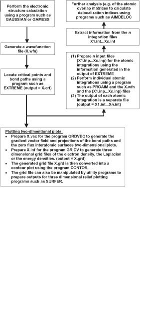
Further, the wavefunction files can be used as input to plotting routines. GRDVEC can be used to generate two-dimensional plots of the gradient vector field and/or the interatomic surfaces and bond paths projected on a plane selected by the user (right half of Fig. 1.3a). Contour diagrams of the density (such as those in the left half of Fig. 1.3a, and Fig. 1.5), the Laplacian, or energy densities can be generated by first calculating the corresponding grid by the use of GRIDV software followed by the generation of the graphics file from the grid

Fig. 1.6 The main steps in a simple QTAIM calculation. The software cited in the figure is part of the AIMPAC suite of programs [129–131]. Other programs are available that can perform most or all of these steps, including, for example, AIM2000 [133–135], MORPHY [132], and AIMALL97 [139].

Appendix 29

by using a program such as CONTOR. (GRDVEC, GRIDV, and CONTOR are components of AIMPAC [129–131]).

The grid generated by GRIDV can be manipulated by utility programs such as GridV_REFORMATTER (available from the authors) to generate inputs for programs such as Surfer [138] which produce three-dimensional relief maps of the field represented by the calculated grid (Fig. 1.1b is an example).

The main steps of a typical QTAIM calculation are summarized in Fig. 1.6.

Appendix: The Inexact Satisfaction of the Molecular Virial Theorem in Electronic Structure Calculations

For a molecule in an equilibrium geometry (with vanishing forces on the nuclei), the molecular virial theorem is expressed as:

V	¼ 2	ð45Þ
g ¼ T

Because of the propagation of numerical errors, small (but non-vanishing) thresholds of convergence of both the SCF and the geometry optimization steps, and the use of incomplete basis sets, electronic structure calculations do not usually satisfy the virial theorem exactly and the virial ratio ðgÞ can deviate by perhaps as much as 0.01 from the ideal value of 2. As a result of this deviation, atomic energies will not sum to yield the molecular energy with acceptable accuracy.

Atomic integration software such as PROAIM [129–131] correct for this error numerically. Thus, instead of simply multiplying each atomic kinetic energy TðWÞ by ð 1Þ to obtain the total atomic energy EðWÞ, the latter is obtained by multiplying TðWÞ by ð1 gÞ. These corrected atomic energies do satisfy Eq. (37), and their sum equals the total molecular energy to within a small numerical integration error. The virial corrections usually scale linearly with regard to TðWÞ which, fortunately, leaves the relative stabilities of the atoms unchanged.

The integration software obtains the virial ratio from the wavefunction files generated by Gaussian [61] or GAMESS [128]. The virial is printed in the last line in the wavefunction file. For Hartree–Fock or density functional calculations, Gaussian prints the correct virial in the wavefunction file and the integrations proceed without problems. For wavefunction files calculated at a post Hartree– Fock level, for example those obtained using Møller–Plesset perturbation theory (MPn) or configuration interaction methods (CI), the virial printed in the wavefunction file generated using the Gaussian 98 or 03 [61] programs (which are available at the time of writing) is the Hartree–Fock virial and not that of the current post- Hartree–Fock method [even if the key word ‘‘DENSITY ¼ CURRENT’’ is invoked and despite the fact that the correct (current) wavefunction is printed]. If such a wavefunction file is fed directly to an integration program, the calculated atomic energies will be rectified using the Hartree–Fock g (instead of the post Hartree– Fock g), resulting in atomic energies which do not add up to the molecular value.

30 1 An Introduction to the Quantum Theory of Atoms in Molecules

In these circumstances the user must calculate the virial of the current method ‘‘by hand’’ from information contained in the Gaussian ‘‘log’’ or ‘‘out’’ output file [140], by dividing, for example, the MP2 (or other correlated total energy) by the kinetic energy listed just after the final electrical multipoles in the Gaussian output. The wavefunction files must then be edited to reflect this new ‘‘correct’’ virial before submitting it to the integration software [140].

In highly accurate calculations it is sometimes necessary to perform atomic integrations of energy densities obtained from systems which satisfy the molecular virial theorem exactly [16, 141]. The author of Chapter 3 of this book, Dr Todd A. Keith, has written a link [142] for Gaussian [61] implementing Lo¨wdin’s selfconsistent virial scaling (SCVS) [143, 144] which produces final wavefunctions satisfying the virial theorem to a very high accuracy.

Acknowledgments

We thank Professor George Heard (University of North Carolina at Asheville) and Dr Katherine N. Robertson (Dalhousie University) for their helpful comments on this chapter, and Dr Todd Keith (Semichem, Inc.) and Dr Jamie Platts (Cardi University) for discussions on the virial correction. The American Chemical Society is acknowledged for its permission to reproduce Fig. 1.5.

References

1	R. F. W. Bader, Atoms in Molecules: A	10	A. Taylor, C. F. Matta, R. J. Boyd,
	Quantum Theory, Oxford University		submitted for publication 2006.
	Press: Oxford, U.K., 1990.	11	R. F. W. Bader, J. A. Platts, J. Chem.
2	P. Coppens, X-ray Charge Densities		Phys. 1997, 107, 8545–8553.
	and Chemical Bonding, Oxford Uni-	12	R. F. W. Bader, Phys. Rev. B 1994, 49,
	versity Press, Inc.: New York, 1997.		13348–13356.
3	P. L. A. Popelier, Atoms in Molecules:	13	J. Schwinger, Phys. Rev. 1951, 82,
	An Introduction, Prentice Hall:		914–927.
	London, 2000.	14	R. F. W. Bader, J. Phys. Chem. A 1998,
4	C. F. Matta, N. Castillo, R. J. Boyd, J.		102, 7314–7323.
	Phys. Chem. A 2005, 109, 3669–3681.	15	T. A. Keith, R. F. W. Bader, Y. Aray, Int.
5	N. Castillo, C. F. Matta, R. J. Boyd,		J. Quantum Chem. 1996, 57, 183–198.
	Chem. Phys. Lett. 2005, 409, 265–269.	16	C. F. Matta, J. Herna´ndez-Trujillo,
6	C. Gatti, P. Fantucci, G. Pacchioni,		T. H. Tang, R. F. W. Bader, Chem.
	Theor. Chem. Acc. (Formerly, Theoret.		Eur. J. 2003, 9, 1940–1951.
	Chim. Acta) 1987, 72, 433–458.	17	C. F. Matta, Chapter 9 in: Hydrogen
7	W. L. Cao, C. Gatti, P. J. MacDougall,		Bonding – New Insight, (S. J.
	R. F. W. Bader, Chem. Phys. Lett.		Grabowski, Ed.), Springer: 2006,
	1987, 141, 380–385.		pp 337–376.
8	M. Sakata, Acta Cryst. A 1990, 46,	18	R. F. W. Bader, C. F. Matta, J. Phys.
	263–270.		Chem. A 2004, 108, 8385–8394.
9	R. Y. de Vries, W. J. Briels, D. Feil, G.	19	R. P. Sagar, A. C. T. Ku, V. H. Jr.
	te Velde, E. J. Baerends, Can. J.		Smith, A. M. Simas, J. Chem. Phys.
	Chem. 1996, 74, 1054–1058.		1988, 88, 4367–4374.

			References	31
20	Z. Shi, R. J. Boyd, J. Chem. Phys.	41	D. Cremer, E. Kraka, Angew. Chem.
	1988, 88, 4375–4377.		Int. Ed. Engl. 1984, 23, 627–628.
21	R. W. F. Bader, G. L. Heard, J. Chem.	42	X. Fradera, M. A. Austen, R. F. W.
	Phys. 1999, 111, 8789–8797.		Bader, J. Phys. Chem. A 1999, 103,
22	R. J. Gillespie, R. S. Nyholm, Quart.		304–314.
	Rev. Chem. Soc. 1957, 11, 339.	43	R. F. W. Bader, M. E. Stephens, J. Am.
23	R. J. Gillespie, R. S. Nyholm, in:		Chem. Soc. 1975, 97, 7391–7399.
	Progress in Stereochemistry (W. Klyne,	44	C. F. Matta, AIMDELOC (QCPE
	P. B. D. de la Mare, Eds.),		0802) Quantum Chemistry Program
	Butterworths: London, 1958.		Exchange, Indiana University, 2001.
24	R. J. Gillespie, I. Hargittai, The		(http://qcpe.chem.indiana.edu/).
	VSEPR Model of Molecular Geometry,	45	Y.-G. Wang, C. F. Matta, N. H.
	Allyn and Bacon: Boston, 1991.		Werstiuk, J. Comput. Chem. 2003, 24,
25	R. F. W. Bader, P. J. MacDougall,		1720–1729.
	C. D. H. Lau, J. Am. Chem. Soc. 1984,	46	Y.-G. Wang, N. H. Werstiuk,
	106, 1594–1605.		J. Comput. Chem. 2003, 24, 379–385.
26	R. F. W. Bader, R. J. Gillespie, P. J.	47	M. A. Austen, A New Procedure for
	MacDougall, J. Am. Chem. Soc. 1988,		Determining Bond Orders in Polar
	110, 7329–7336.		Molecules, with Applications to
27	R. J. Gillespie, I. Bytheway, T.-H.		Phosphorus and Nitrogen Containing
	Tang, R. F. W. Bader, Inorg. Chem.		Systems, Ph.D. Thesis, McMaster
	1996, 35, 3954–3963.		University: Hamilton, Canada, 2003.
28	M. T. Carroll, C. Chang, R. F. W.	48	C. F. Matta, J. Herna´ndez-Trujillo,
	Bader, Mol. Phys. 1988, 63, 387–405.		J. Phys. Chem. A 2003, 107, 7496–
29	M. T. Carroll, J. R. Cheeseman, R.		7504 (Correction: J. Phys. Chem. A
	Osman, H. Weinstein, J. Phys. Chem.		2005, 109, 10798).
	1989, 93, 5120–5123.	49	E. A. Zhurova, C. F. Matta, N. Wu,
30	R. J. Boyd, S. C. Choi, Chem. Phys.		V. V. Zhurov, A. A. Pinkerton, J. Am.
	Lett. 1986, 129, 62–65.		Chem. Soc. 2006, 128, 8849–8861.
31	M. T. Carroll, R. F. W. Bader, Mol.	50	R. F. W. Bader, P. F. Zou, Chem.
	Phys. 1988, 65, 695–722.		Phys. Lett. 1992, 191, 54–58.
32	E. Espinosa, E. Molins, C. Lecomte,	51	C. F. Matta, R. F. W. Bader, J. Phys.
	Chem. Phys. Lett. 1998, 285, 170–173.		Chem. A 2006, 110, 6365–6371.
33	S. J. Grabowski, J. Phys. Chem. A	52	(a) L. Cohen, J. Chem. Phys. 1979, 70,
	2001, 105, 10739–10746.		788–789; (b) L. Cohen, J. Chem. Phys.
34	M. Domagala, S. Grabowski, K.		1984, 80, 4277–4279.
	Urbaniak, G. Mloston, J. Phys. Chem.	53	F. Corte´s-Guzma´n, J. Herna´ndez-
	A 2003, 107, 2730–2736.		Trujillo, G. Cuevas, J. Phys. Chem. A
35	S. Grabowski, W. A. Sokalski,		2003, 107, 9253–9256.
	J. Leszczynski, J. Phys. Chem. A 2005,	54	R. F. W. Bader, J. R. Cheeseman, K. E.
	109, 4331–4341.		Laidig, K. B. Wiberg, C. Breneman,
36	M. Domagala, S. Grabowski, J. Phys.		J. Am. Chem. Soc. 1990, 112,
	Chem. A 2005, 109, 5683–5688.		6530–6536.
37	O. Knop, R. J. Boyd, S. C. Choi,	55	R. F. W. Bader, C. F. Matta, Int. J.
	J. Am. Chem. Soc. 1988, 110, 7299–		Quantum Chem. 2001, 85, 592–607.
	7301.	56	C. F. Matta, Applications of the
38	J. L. Jules, J. R. Lombardi, J. Mol.		Quantum Theory of Atoms in Molecules
	Struct. (Theochem) 664–665, 2003,		to Chemical and Biochemical Problems,
	255–271.		Ph.D. Thesis, McMaster University:
39	S. T. Howard, O. Lamarche, J. Phys.		Hamilton, Canada, 2002. (Available
	Org. Chem. 2003, 16, 133–141.		on line, http://chem.utoronto.ca/
40	R. F. W. Bader, T. T. Nguyen-Dang,		~cmatta/).
	Adv. Quantum Chem. 1981, 14,	57	C. F. Matta, R. J. Gillespie, J. Chem.
	63–124.		Educ. 2002, 79, 1141–1152.