Matta, Boyd. The quantum theory of atoms in molecules

102 4 QTAIM Analysis of Raman Scattering Intensities

Fig. 4.3 Comparison with experimental values of mean molecular polarizability calculated at the HF/D95(d,p) level. Data from Refs. [22, 27].

racy to reproduce experimentally observed trends. Much of our early work was successful with the lower level HF/D95(d,p) calculations (Fig. 4.3) [21, 27]. For those readers who are interested in pushing the limits of accuracy, in Section 4.4 we present a detailed example of a high-level calculation that will match experimental data.

Having verified that acalc is satisfactory, we approximate qa=qr by finite di erence:

	qr	ADr		¼ n		2Dr		ð		Þ
	qa		Da	1		aþDr a Dr			4
where the change in bond length, Dr, is typically G1:00 10 12								m; n ¼ number

of symmetrically equivalent bonds stretched or contracted, and aGDr denotes the mean molecular polarizability at the stretched or contracted geometry. The accuracy of the central-di erence derivative formula is second-order in step size; we have confirmed that good values are produced even for steps of Dr ¼ 1:00 10 11 m [28]. The step size that we recommend here is a typically accepted value for this type of finite di erence model.

4.3.2

Recouping a From the Wavefunction, With QTAIM

According to QTAIM, the dipole induced by the applied field is the result of charge transfer (CT) between atomic basins and changes in atomic dipole (AD)

4.4 Specific Examples of the Use of AIM2000 Software to Analyze Raman Intensities 103

within a basin. In practical terms, ai; jðWÞ, the atomic contribution to the i, jth entry in the polarizability tensor, is expressed as:

	a	i; jð	W	Þ ¼		ðNi N0Þrj	þ	mi m0	5	Þ
						Ei		Ei
									ð

where Ni and N0 are the atomic electron populations when E is applied in the ith direction and when E ¼ 0, respectively, for atom W located at rj ð j ¼ x; y; zÞ. Atomic population is the atomic number minus the charge. The AD term is found from the change in the atomic first moment, m, with and without the applied field. The ai; jðWÞ are summed over all atoms to give the molecular tensor a.

4.3.3

Recovering qa/qr From QTAIM

In other chapters we have seen the incredible insight into structure and its underlying basis, bonding, gained by QTAIM analyses. In essence, this approach puts skin on the bones of the molecular skeleton; we want, however, to animate our understanding of bonding, to go beyond the question of static equilibrium structure and delve into the response of the molecule to perturbation, as seen in the changes in the topology of the electron density. Short of ionization, we know that the electrons will remain in the molecule. This is rather unsatisfying. We can look a little more deeply and report that, in the presence of a perturbing laser field, the electrons would redistribute themselves within the molecule. As in the static example, an atomic-level description is convenient and powerful, and provides a rigorous connection between theory and experiment. The picture now becomes one of electronic flow throughout a molecule and of reorientation of charge within atoms.

The recovery of the derivative from the wavefunctions that we have created is a straightforward process, based on Eqs (4) and (5). For each atom, we can examine:

qai; j	G	Dai; jðWÞ ðNi N0Þrj				mi m0	6
qr		Dr	¼	Dr Ei	þ	Dr Ei	ð	Þ

The right hand side of the equation quantifies the changes in the CT and AD terms at each atom ðDCTðWÞ=Dr and DADðWÞ=DrÞ, in response to the molecular vibration and the applied field. We will discuss the patterns and trends that QTAIM reveals in Sections 4.5 ðaÞ and 4.6 ðqa=qrÞ.

4.4

Specific Examples of the Use of AIM2000 Software to Analyze Raman Intensities

We next carry out the step-by-step procedure of Raman intensity analysis through QTAIM for H2 and CH4. These molecules are small enough to enable excellent

104 4 QTAIM Analysis of Raman Scattering Intensities

calculations relatively quickly while still demonstrating the major outcomes. It is important to distinguish between the accuracy or method of the calculation and the actual convergence level of that chosen method. When a is computed numerically (through energy or dipole derivatives) using small applied fields, the results are sensitive to the SCF convergence, especially when the derived polarizabilities are computed from small displacements in bond lengths, chosen to better approximate qa=qr. On the basis of error analysis, we recommend a computationally inexpensive SCF convergence of 10 11 rather than 10 8, a typical default value.

4.4.1

Modeling a in H2

For H2 with only two electrons and one geometric parameter, it is possible to perform a very high-level calculation on an ordinary PC; CCSD for a two-electron system is equivalent to the full configuration interaction method. With that, we use the aug-cc-pVQZ basis set, a large correlation consistent basis (quadruple zeta) with di use and polarization functions. The CCSD value of a ¼ 0:856 10 40 Cm2 V 1 compares very well with experiment (0:858 10 40 Cm2 V 1) [29], as per our check of Step 1. Following Steps 2 and 3, we obtain a CCSD value for Da=Dr of 1:36 10 30 Cm V 1, again in excellent agreement with several experimental values (1:36 10 30 Cm V 1) [30].

For the QTAIM calculations we use E ¼ 0.001 au, the same field strength as in the numerical CCSD Gaussian calculation, to facilitate direct comparisons. It is small enough to minimize the e ect of higher-order polarizabilities, and tends to give excellent agreement with analytical (CPHF) calculations where the method allows. One must usually compute wavefunctions for E0 ¼ 0 and with fields Ex, Ey, and Ez, for each geometry, and average the results obtained from fields applied in both directions along each axis. For H2 we had aligned the principal axis (bond axis) with the z-axis, thereby diagonalizing the polarizability tensor and making axx ¼ ayy. Thus for each unique geometry (Dr ¼ 0,G1:00 10 12 m), we need only to compute a reference wavefunction file with E0, Ex , and Ez applied fields (the þ and directions being equivalent).

It must be stressed that analysis of Raman intensities requires the maximum accuracy from QTAIM integrations, because we are looking for the e ects of very small perturbations (electrostatic and geometric) on the atomic electronic properties. A relatively small error of 10 3 au in mðWÞ becomes an error of 1 au in aðWÞ, in turn producing huge errors in the calculated qa=qr; any insights gained would be suspect. With AIM2000 we have found the greatest accuracy to be obtained by integrating in ‘‘natural coordinates’’. We set the relative and absolute integration accuracy values to 1 10 6, which are two orders of magnitude tighter than the default and is at the limit of the numerical stability of the current implementation. The beta-sphere radius is set equal to the distance from the nuclear attractor (NA) (not necessarily exactly at the nuclear position) to the nearest bond critical point. Finally we triple the default maximum path length ‘‘s’’ to

4.4 Specific Examples of the Use of AIM2000 Software to Analyze Raman Intensities 105

Table 4.1 QTAIM integration results for H2 at equilibrium geometry (in atomic units).

	W	Atomic charge	mx	my	mz	Atomic energy
E0	H1	0.0002989	0.0000047	0.0001498	0.0945175	0.5666
	H2	0.0003008	0.0000004	0.0001436	0.0945188	0.5666
Ex	H1	0.0002061	0.0023122	0.0001386	0.0944551	0.5667
	H2	0.0002049	0.0023128	0.0001412	0.0944540	0.5667
Ez	H1	0.0041055	0.0000028	0.0001437	0.0946650	0.5683
	H2	0.0046799	0.0000005	0.0001420	0.0943614	0.5650

3 106. The path length has never been a limiting factor for the molecules considered. With these values it is common to recover a to better than 99%; this level of completeness enables, at the very least, semi-quantitative recovery of Raman intensities.

In Table 4.1 we show the integration data for H2 at equilibrium geometry for E0, Ex , and Ez (note that all data are in au unless otherwise stated). For E0, the charge on each atom is zero to within a few parts in 104; the x and y atomic dipoles cancel to within a few parts in 106. Although the z-component of the molecular dipole should be zero, each atom has a non-zero dipole reflecting the shape of the densities around the nuclei; these are equal and opposite. The net magnitude of the molecular dipole is less than 1 10 5. This can be regarded as a highquality integration, because the dipole error would only a ect calculated polarizabilities by 1 10 2. For Ex, symmetry excludes the possibility of charge transfer; only an induced dipole in the x-direction is possible. The x-coordinate of the density maxima (NA) is su ciently distorted by the field to move slightly away from the nuclear position, rx(NA) ¼ 3:586 10 5, rx(H) ¼ 0. This is typical of light atoms. One must be careful to use the position of the NA and not the nucleus when applying the formulas for atomic electronic properties. For Ez ¼ 0.001 au, there is both CT between hydrogen atoms and a nonzero AD (distortion of the density) in each atomic basin. Average atomic contributions to the axx and azz elements, in au, are computed from Eq. (5): CTðWÞxx ¼ 0, ADðWÞxx ¼ 2:312; CTðWÞzz ¼ 2:996, ADðWÞzz ¼ 0:152; after summation and conversion we get aðH2Þ ¼ 0:854 10 40 Cm2 V 1. The atomic average is equivalent to averaging the field in both directions along the axis; we find an excellent QTAIM recovery of 99.7601%.

A word of caution is necessary here. The robustness of electronic structure codes is usually much greater than that of available QTAIM integration software (for the accuracies we require). This means that an electronic structure calculation should always converge to precisely the same energy (and properties) for symmetry-equivalent species. In contrast, the nature of the QTAIM integration

106 4 QTAIM Analysis of Raman Scattering Intensities

grid could produce orientation-dependant results. With our very accurate values we could not find any instances of this, despite using much stronger fields to distort the charge densities, and intentionally integrating in favorable and unfavorable orientations, data not shown.

4.4.1.1Modeling Da/Dr in H2

To complete the analysis of Raman intensities for H2, one must repeat the steps above for stretched and contracted geometries. Our usual approach is to displace the nuclei by 0.01 A˚ ; the error in aQTAIM (less than 2%) is, however, still enough to cause problems with interpretation of qa=qr (QTAIM recovery error of >30%). We repeated the calculation for Dr ¼G0:04 A˚ and obtained much better agreement between GDr, and better overall recovery. The average atomic contributions to a are shown for Dr ¼ þ0:04 A˚ , to highlight the orientation dependence of the changes, i ¼ x; y; z:

x field
DCTðHÞix ¼ ð0:000	0:000 0:002Þ
DADðHÞix ¼ ð0:132	0:002 0:002Þ
z field
DCTðHÞiz ¼ ð0:000	0:000 0:205Þ
DADðHÞiz ¼ ð 0:003	0:004 0:078Þ	ð7Þ

For H2, the perpendicular contribution ðaxx Þ is necessarily entirely AD; CT is the dominant contribution to a along the bond (z axis) and the largest tensor component overall. The recovered value Da=DrQTAIM for H2 (1:48 10 30 Cm V 1) is in reasonable agreement with that calculated in Gaussian (1:36 10 30 Cm V 1), which is identical with the experimental value [30].

4.4.2

Modeling a and Da/Dr in CH4

For this larger system with ten electrons, we have chosen the B3LYP hybrid density functional method with the aug-cc-pVTZ basis set. This is very computationally a ordable for medium and even larger systems. The computed qa=qrCH is in perfect agreement with experiment [31] (Steps 1–3, and below). Another advantage is that analytical polarizabilities are available by use of the CPHF method. This enables us to compare numerical polarizability results obtained from energy or dipole derivatives with the analytical values. With its Td symmetry, methane has only one unique, nonzero polarizability tensor element. We chose to orient the molecule so that the hydrogen atoms appear at the corners of a cube. The QTAIM results for the equilibrium geometry are shown in Table 4.2. The x, y, and z directions are equivalent; our electronic structure calculations produce the same results for all field directions (and are unchanged for a C3v geometry with

4.4 Specific Examples of the Use of AIM2000 Software to Analyze Raman Intensities 107

Table 4.2 QTAIM integration results for methane at equilibrium geometry for E0 and Ex (in atomic units).

	W	Atomic charge	mx	my	mz	Atomic energy
E0	C	0.0219197	0.0004455	0.0000028	0.0000110	38.0411
	H1	0.0053341	0.0854614	0.0853861	0.0853876	0.6243
	H2	0.0049950	0.0860062	0.0855185	0.0854416	0.6241
	H3	0.0050035	0.0860009	0.0855167	0.0854399	0.6241
	H4	0.0053182	0.0854648	0.0853973	0.0853895	0.6243
Ex	C	0.0219291	0.0004116	0.0000410	0.0015141	38.0411
	H1	0.0079645	0.0853935	0.0853224	0.0869203	0.6253
	H2	0.0076480	0.0859373	0.0854687	0.0869380	0.6251
	H3	0.0023261	0.0860613	0.0856022	0.0839633	0.6230
	H4	0.0026376	0.0855481	0.0854562	0.0839168	0.6232

one CH pointed along the z axis, not shown). Thus, we need only perform two QTAIM analyses (E0 and Ez) at each of Dr ¼ 0, G0:01 10 12 m (Table 4.3). The individual CTxz terms are large but cancel on summation, owing to symmetry; individual ADxz terms are quite small, and also cancel. For the zz terms, we see the interesting e ect of CT from one end of the molecule to the other, with no net CT to the carbon atom. Carbon, however, has an AD opposing this e ect, and the hydrogen atoms a large AD terms, reflecting the nonspherical density around each H, in the field direction.

The change in atomic contributions to a at the equilibrium, stretched, and contracted geometries are illustrative of the insights into Raman intensities and charge flow in general that are possible through QTAIM analysis (Table 4.4).

Table 4.3 QTAIM analysis of CT(W) and AD(W) to aiz(CH4) at Ez, Dr ¼ 0 (in atomic units: a0 3).

W CTxz(W)		CTyz(W) CTzz(W) ADx z(W)			ADyz(W) ADzz(W) ax z			ayz	azz
C	0.0	0.0	0.0	0.03386	0.03819 1.52518		0.03386	0.03819	1.52518
H1	3.07854	3.07854	3.07864	0.06794	0.06371	1.53278	3.01060	3.01483	4.61142
H2 3.10500		3.10509	3.10518	0.06883	0.04983	1.49646	3.03617	3.05526	4.60164
H3	3.13346	3.13355	3.13345 0.06038		0.08544	1.47667	3.07308	3.04811	4.61012
H4 3.13723		3.13723	3.13713	0.08329	0.05882	1.47276 3.05395		3.07842	4.60989
SW 0.03023		0.02287 12.45440		0.05766	0.02545	4.45349	0.02743	0.04832	16.90789
B3LYP/aug-cc-pVTZ							0.0	0.0	17.02210
Recovery by QTAIM %							100.027	99.952	99.329

1084 QTAIM Analysis of Raman Scattering Intensities

Table 4.4 QTAIM recovery of a and Da=Dr for CH4, where qa=qr 1qazz=qr.

[a]	˚	B3LYP	QTAIM	Recovery (%)	Expt.
Parameter(units)	Dr(A)
azz (a0 3)	0.01	16.7200	16.5572	99.026
azz (a0 3)		17.0221	16.9079	99.329
azz (a0 3)	þ0.01	17.3288	17.1638	99.048
a (Cm2 V 1)	0	2:807 10 40	2:787 10 40		2.85[b]–
					2.93[c] 10 40
Da=Dr (Cm V 1)		1:245 10 30	1:055 10 30
Da=Drþ (Cm V 1)		1:264 10 30	1:446 10 30
Da=Dr (Cm V 1)	average	1:255 10 30	1:250 10 30	99.64	1:26 10 30[d]

a Conversion factor 1.648777631 10 41 * (a0)3 ¼ Cm2 V 1. b Ref. [27].

c Ref. [33]. d Ref. [32].

The average atomic contributions for the Ez field at Dr ¼ 0 are:

CTizðCÞ ¼ ð0 0 0Þ
CTizðHÞ ¼ ð 0:008	0:006	þ3:114Þ
ADizðCÞ ¼ ðþ0:034	0:038	ð8Þ
		1:525Þ
ADizðHÞ ¼ ð 0:002	0:003	þ4:608Þ

A significant contribution to Da=DrCH is the decrease in the opposing AD in the carbon atom by 0.045 au along with increases in CT(H) and AD(H). This type of analysis for systems with unusual charge flow (reflected in the Raman intensities) will reveal the structural factors that govern the most extreme behavior.

4.4.3

Additional Exercises for the Interested Reader

Given the limitations in QTAIM integration accuracy, it is important to establish the best geometric step size for studying ðqa=qrÞ. Using the data provided below, compute ðDa=DrÞ for methane and H2 using the first-order accurate forward– di erence method for:

(a)stretched and equilibrium geometry, and

(b)equilibrium and contracted geometry. Answers:

(a)H2: 1.362 10 30 Cm V 1 methane: 1.264 10 30 Cm V 1; and

(b)H2: 1.352 10 30 Cm V 1 methane: 1.245 10 30 Cm V 1

4.5 Patterns in a That Are Discovered Through QTAIM 109

Compare these results with those from the second-order accurate centraldi erence method using the stretched and contracted data.

Answers: H2 Da=Dr: 1.357 10 30 Cm V 1 methane: 1.255 10 30 Cm V 1 Compute the second derivatives using the three-point second-derivative for-

mula and the data below.

Answers: H2: 9.735 10 21 C V 1 methane: 1.895 10 21 C V 1.

Run electronic structure calculations computing polarizabilities for methane and H2 at larger bond displacements (e.g. G0.02 A˚ , G0.04 A˚ , . . . G0.1 A˚ ).

How do the values obtained for ðDa=DrÞ compare with those from the smaller step size? What is the largest step-size that preserves ðDa=DrÞ to within 2%? Could the largest accurate step-size be estimated from the small step-size secondderivative result?

Data: a (au) at Contracted/Equilibrium/Stretched geometries (G0.01 A˚ ) H2: 5.113/5.195/5.277.

Methane: 16.720/17.022/17.329.

4.5

Patterns in a That Are Discovered Through QTAIM

Molecular polarizability to describes the displacement of the electrons in a molecule when it is placed in an electric field. In the language of QTAIM, this displacement has two parts: transfer of charge from one atomic basin to another and polarization of charge within an atomic basin. The challenge for us is that the properties we are examining are extraordinarily sensitive to our (in)ability to numerically recover the full information available in the wavefunction. It is important to emphasize that this is a numerical and implementation problem rather than a fundamental problem with the QTAIM theory. Fortunately, we do not have to push the calculation levels to the limit in Section 4.4 to uncover these patterns. The results are worthwhile, as is seen in the QTAIM analysis of the polarizabilities of the simple alkanes, for example methane, ethane, and propane [17]. Initially, we only used the D95(d,p) basis at the HF level, yet we discovered the patterns of behavior [17–21] identical with those revealed in Section 4.4 and calculated with larger basis sets [27]. In ethane and propane we see the emergence of the patterns in a that underlie those in qa=qr [17].

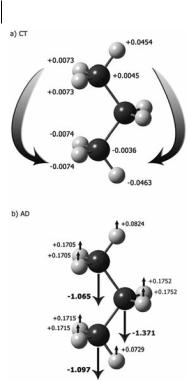
In Fig. 4.4, we see the e ect of Ez on propane. Just as in CH4, the CT term is greatest along the field axis and is essentially a transfer between the atoms at the extreme ends of the molecule. In propane, these are the H atoms that lie in the skeletal plane, denoted Hip (ip ¼ in plane). There is a smaller though still significant transfer between the methyl hydrogen atoms that lie out of the plane, denoted Hop (op ¼ out of plane) and between the terminal methyl carbons. The methylene group (CHm) does not participate. As might be expected, integration over the atomic basins of each atom shows that the charge is transferred symmetrically, creating a CT dipole that opposes the applied field. The story changes when we examine the atomic dipoles. The AD(H) are aligned with those created

110 4 QTAIM Analysis of Raman Scattering Intensities

Fig. 4.4 QTAIM analysis of response for an electric field applied to propane in the z direction. (a) Charge transfer (CT) and (b) atomic dipole (AD) contributions (10 40 Cm2 V 1) to the azz term in the molecular polarizability of propane. By convention, the z-axis is defined as the axis with maximum polarizability. Data were calculated at the HF/D95(d,p) level, from Ref. [17].

through CT. However, the ADs of all three Cs that form the inner skeleton of the molecule are directed in the opposite sense. The molecular polarizability is the net result of these opposing contributions.

We found the identical pattern in each field direction and in every molecule we have analyzed with QTAIM. The amount of charge transferred between terminal H atoms increases with chain length, while the opposing ADs in the carbon skeleton also increase [19]. In cyclohexane [18], when the field is applied along the nominal ring plane, the CT(Heq) terms are very large. For the field perpendicular to the ring plane, the CT between the Hax is significant; the CT contribution in Eqs. (5) and (6) is still smaller, however, because the distance over which the charge is transferred is smaller. The picture that emerges is similar to the surface charge polarization of an idealized dielectric body of uniform positive and negative charges. The surface polarization overrides the e ect of the external field on the interior. The CT on the outer H atoms is countered by an AD formed by reorganization of charge within the carbon atomic basins.

4.6 Patterns in qa/qrCH That Apply Across Di erent Structures, Conformations, Molecular Types 111

4.6

Patterns in qa/qrCH That Apply Across Di erent Structures, Conformations, and Molecular Types: What is Transferable?

In this section, the emphasis is focused on the dynamic nature of qa=qr compared with the more static nature of the polarizability. In exploring qa=qr, we seek local details rather than merely global information and QTAIM provides the means with which to examine the molecular wavefunction. The derivatives are not transferable, so what is? The answer lies in the patterns revealed by QTAIM analysis.

Experimental data on absolute Raman trace scattering intensities are the acid test for the validity of the theoretical models; such experiments are tractable, however, only for small, highly symmetrical molecules that can be studied easily in the gas phase. Experimental qa=qr have been obtained for methane, ethane, propane, butane, cyclohexane, ethene, ethyne, and, most recently, for bicyclo- [1.1.1]-pentane [6, 8–13]. Relative values for qa=qrCH have been determined for n-pentane, which occurs as a mixture of trans–trans, gauche–trans and gauche– gauche conformers in the gas phase at room temperature [19]. Our detailed QTAIM analyses have been directed to these molecules. We have also completed survey studies, Steps 1–3 above, on over 50 molecules, to identify trends in calculated Da=Dr values and to find appropriate candidates for further detailed experimental and theoretical analysis [20–22].

4.6.1

Patterns in Da/DrCH Revealed by QTAIM

From our QTAIM analysis, we have seen that alkanes behave like tiny pieces of polarizable material, with end-to-end transfer of charge opposed by internal dipoles. Although this behavior can be trivially understood in a gross sense, what is of greater interest is to understand the e ect of the molecular framework on the flow of charge and the rearrangement of atomic electron densities. We are studying the behavior of a charge cloud bound by nuclear attractors and distributed across distinct atomic basins. With the data in hand we can now explore the dynamics of the electron density during a molecular vibration.

4.6.1.1QTAIM Analysis of Da/DrCH in Small Alkanes

Complete QTAIM analysis has been conducted for methane, ethane, propane, the trans, trans conformation of n-pentane, and cyclohexane [17–19]. The first thing we note is that the change in a, the mean molecular polarizability associated with the stretch of any CH bond, arises from changes distributed throughout the molecule [17–19]. The complexity of the response is illustrated for the three di erent CH stretch modes in propane (Fig. 4.5) [17]. The numbers beside each atom are the atomic contributions (Eq. 6) divided by the number of equivalent bonds, to give DaðWÞ=DrCH, i.e. the derivative per CH bond (all Da=Dr are reported in units of 10 30 Cm V 1). The contributions are largest for the atoms of the bond being stretched, but the contributions from the remainder of the molecule cannot be