Matta, Boyd. The quantum theory of atoms in molecules

232 9 Atoms in Molecules Theory for Exploring the Nature of the Active Sites on Surfaces

ated to ‘rðrÞ ¼ 0. The NR algorithm requires evaluation of the first and second partial derivatives of r, at arbitrary points r.

The points of the necessary gradient paths to determine the bond paths, crystal graphs, and IAS are solutions of the di erential equation [1]:

drðsÞ=ds ¼ ‘rðrðsÞÞ

ð2Þ

where the notation rðsÞ implies that a point r on a given path is dependent upon the path parameter s. Equation (2) represents three first-order di erential equations (dxiðsÞ=ds ¼ qr=qxi, xi ¼ x; y; z) and yields unique solutions only when particular values are assigned to three constants of integration. This corresponds to fixing some initial point on a trajectory, at s ¼ s1, for example. A trajectory of the gradient vector field of r(r) is a parametrized integral curve, a solution curve, of the di erential equation for ‘r(r). By fixing a point on a given trajectory all other points which lie on the same path, can be obtained by solving Eq. (2). This is achieved by using a fifth-order Cash–Karp Runge–Kutta (CKRK) method [12]. The general form of the Runge–Kutta formula is:

xnþ1 ¼ xn þ c1k1 þ c2k2 þ c3k3 þ c4k4 þ c5k5 þ c6k6

ð3Þ

where xn ¼ ðxn; yn; znÞ and kj over an interval h are:

k1 ¼ h‘rðrÞjr¼xn

k2 ¼ h‘rðrÞjr¼xn þb21k1

k6 ¼ h‘rðrÞjr¼xn þb61k1 þ þb65k5

The particular values of the various constants ðcj; bijÞ are given in Ref. [12].

It is apparent the key for implementation of the NR and CKRK algorithms is calculation of the required derivatives of r(r), at arbitrary points r. To develop a method enabling us to study complex systems, irrespective of the basis set (analytically or numerically) used, a numerical method on electron densities given on regular, not necessarily homogeneous three-dimensional grids was implemented. The necessary partial derivatives are evaluated using a five-degree Lagrange polynomial interpolation of r(r) and are fed into an automated algorithm for systematic determination of the all CPs. For just one dimension the interpolating polynomial of degree n 1 through n points y1 ¼ f ðx1Þ, y1 ¼ f ðx1Þ; . . . ; yn ¼ f ðxnÞ is given by the Lagrange’s formula:

			n
n		j	Y1; j0kðx xjÞ
PðxÞ ¼ Xk 1			¼	yk	ð4Þ
			n
¼	j		Y1; j0kðxk xjÞ
		¼

9.2 Implementing the Determination of the Topological Properties of rðrÞ	233

There are n terms, each a polynomial of degree n 1 and each constructed to be zero at all xj except one, at which it is constructed to be yk. For a homogeneous grid, xj ¼ x1 þ ð j 1Þh, where h is the step size. Defining s ¼ ðx xaÞ=h so that xa and xaþ1 are the central points of the grid, we obtain x ¼ xa þ sh. Substituting this last expression in Eq. (4) we have:

				n
n	j		Y1; j0kða j þ sÞ
P ¼ Xk 1		¼					yk		ð5Þ
					n
¼			j	Y1; j0kðk jÞ
				¼
and
n
P ¼ Xk 1 wk; nðsÞ yk									ð6aÞ
¼
where
					n
			j	Y1; j0kða j þ sÞ
wk; nðsÞ ¼				¼					ð6bÞ
					n
				j	Y1; j0kðk jÞ
					¼

wk; nðsÞ are polynomials of degree n 1 in s. The n-degree derivative of these expressions is:

dvP			1			n
		¼			Xk 1 wkðv; ÞnðsÞ yk
dx v				hv
					¼			ð7Þ
wðvÞ					dvwk; nðsÞ
		s
k; n		ð	Þ ¼			dsv

Equations (6) and (7) provide an accurate, rapid, and e cient way of interpolating r(r) and its derivatives at many arbitrary points. The easiest way to determine those derivatives is to develop wk; nðsÞ as an s polynomial. For example, in Table 9.1 the s polynomial expression for wk; nðsÞ and its first and second derivatives for interpolation with n ¼ 4; 6, and 8 points are reported. The explicit expression for n ¼ 4 (Fig. 9.1) is given by:

rðxÞ ¼ ð s3 þ 3s2 2sÞ=6r1 þ ðs3 2s2 s þ 2Þ=2r2
þ ð s3 þ s2 þ 2sÞ=2r3 þ ðs3 sÞ=6r4	ð8Þ

For a three-dimensional system P is evaluated at points surrounding a box containing the current point and in such a way that any coordinates of the point

Table 9.1	wðvÞ	ðsÞ polynomial defined using Eqs (6) and (7), with a ¼ n=2 and w			ðsÞ ¼ wð0Þ	ðsÞ.
	k, n			k, n	k, n
			n F 4	n F6			n F8
v ¼ 0		k ¼ 1	ðs3 þ 3s2 2sÞ=6	ðs5 þ 5s4 5s3 5s2 þ 6sÞ=120			ðs7 þ 7s6 7s5 35s4 þ 56s3 þ 28s2 48sÞ=5040
		k ¼ 2	ðs3 2s2 s þ 2Þ=2	ðs5 4s4 s3 þ 16s2 12sÞ=24			ðs7 6s6 2s5 þ 60s4 71s3 54s2 þ 72sÞ=720
		k ¼ 3	ðs3 þ s2 þ 2sÞ=2	ðs5 þ 3s4 þ 5s3 15s2 4s þ 12Þ=12			ðs7 þ 5s6 þ 9s5 65s4 þ 16s3 þ 180s2 144sÞ=240
		k ¼ 4	ðs3 sÞ=6	ðs5 2s4 7s3 þ 8s2 þ 12sÞ=12			ðs7 4s6 14s5 þ 56s4 þ 49s3 196s2 36s þ 144Þ=144
		k ¼ 5		ðs5 þ s4 þ 7s3 s2 6sÞ=24			ðs7 þ 3s6 þ 17s5 39s4 88s3 þ 108s2 þ 144sÞ=144
		k ¼ 6		ðs5 5s3 þ 4sÞ=120			ðs7 2s6 18s5 þ 20s4 þ 89s3 18s2 72sÞ=240
		k ¼ 7					ðs7 þ s6 þ 17s5 5s4 64s3 þ 4s2 þ 48sÞ=720
v ¼ 1		k ¼ 8	ð3s2 þ 6s 2Þ=6	ð5s4 þ 20s3 15s2 10s þ 6Þ=120			ðs7 14s5 þ 49s3 36sÞ=5040
		k ¼ 1					ð7s6 þ 42s5 35s4 140s3 þ 168s2 þ 56s 48Þ=5040
		k ¼ 2	ð3s2 4s 1Þ=2	ð5s4 16s3 3s2 þ 32s 12Þ=24			ð7s6 36s5 10s4 þ 240s3 213s2 108s þ 72Þ=720
		k ¼ 3	ð3s2 þ 2s þ 2Þ=2	ð5s4 þ 12s3 þ 15s2 30s 4Þ=12			ð7s6 þ 30s5 þ 45s4 260s3 þ 48s2 þ 360s 144Þ=240
		k ¼ 4	ð3s2 1Þ=6	ð5s4 8s3 21s2 þ 16s þ 12Þ=12			ð7s6 24s5 70s4 þ 224s3 þ 147s2 392s 36Þ=144
		k ¼ 5		ð5s4 þ 4s3 þ 21s2 2s 6Þ=24			ð7s6 þ 18s5 þ 85s4 156s3 264s2 þ 216s þ 144Þ=144
		k ¼ 6		ð5s4 15s2 þ 4Þ=120			ð7s6 12s5 90s4 þ 80s3 þ 267s2 36s 72Þ=240
		k ¼ 7					ð7s6 þ 6s5 þ 85s4 20s3 192s2 þ 8s þ 48Þ=720
v ¼ 2		k ¼ 8	s þ 1	ð2s3 þ 6s2 3s 1Þ=12			ð7s6 70s4 þ 147s2 36Þ=5040
		k ¼ 1					ð3s5 þ 15s4 10s3 30s2 þ 24s þ 4Þ=360
		k ¼ 2	3s 2	ð10s3 24s2 3s þ 16Þ=12			ð21s5 90s4 20s3 þ 360s2 213s 54Þ=360
		k ¼ 3	3s þ 1	ð10s3 þ 18s2 þ 15s 15Þ=6			ð7s5 þ 25s4 þ 30s3 130s2 þ 16s þ 60Þ=40
		k ¼ 4	s	ð10s3 12s2 21s þ 8Þ=6			ð21s5 60s4 140s3 þ 336s2 þ 147s 196Þ=72
		k ¼ 5		ð10s3 þ 6s2 þ 21s 1Þ=12			ð21s5 þ 45s4 þ 170s3 234s2 264s þ 108Þ=72
		k ¼ 6		ð2s3 3sÞ=12			ð7s5 10s4 60s3 þ 40s2 þ 89s 6Þ=40
		k ¼ 7					ð21s5 þ 15s4 þ 170s3 30s2 192s þ 4Þ=360
		k ¼ 8					ð3s5 20s3 þ 21sÞ=360

Surfaces on Sites Active the of Nature the Exploring for Theory Molecules in Atoms 9 234

9.2 Implementing the Determination of the Topological Properties of rðrÞ	235

Fig. 9.1 One-dimensional example of the interpolation at x with n ¼ 4 points, xi and ri are the abscissa and density values at grid point i.

x are at the center of the points arrangement. The interpolation is accomplished by a sequence of one-dimensional interpolations. For example, on a Cartesian mesh (Fig. 9.2) of tabulated values yk (black circles) such as a parallelepiped, a two-dimensional square-mesh with approximated yi (dark gray circles in Fig. 9.2)

Fig. 9.2 Example of the interpolation method for a three-dimensional mesh of points. Black circles denote the points with tabulated values of the function. The open circle denotes the current point where the function must be interpolated. (a) A square of interpolated values at points denoted by gray circles is obtained applying the one-dimensional Lagrange interpolation to each line of

six points along the black arrows. (b) and

(c) show the square array after the first approximation. In (c) the light circles denote a new approximation using four-point linear interpolation along the black arrows. Finally, using a one-dimensional interpolation on the light gray line, the approximation of the function at the current value is obtained.

236 9 Atoms in Molecules Theory for Exploring the Nature of the Active Sites on Surfaces

values on a plane that coincides with just one of the coordinates of the current point (open circle) is determined. Then, on the plane, a linear mesh (Fig. 9.2c) that coincides with an additional coordinate of the current point is approximated. Finally, the value of P is interpolated on this linear arrangement.

The final equation is:

n1	n2	n3
P ¼ kX1 1 kX2 1 kX3 1 wk1; n1 ðs1Þ wk2 ; n2 ðs2Þ wk3; n3 ðs3Þ yk1k2k3			ð9Þ
¼	¼	¼

Taking advantage of the crystal symmetry and the properties of the gradient paths of r(r) associated with the CPs, we have implemented a very rapid, automated algorithm for systematic determination of the all CPs inside the unit cell of the crystal. First, it determines the bond CP among each pair of atoms (first and second neighbors) using the NR method. Because the gradient paths associated with the negative eigenvalues at the bond CPs originate mainly in the cage CPs, the algorithm then simply searches the origin of some of these paths (for each bond CP) applying the NR method at these points. Finally, searching along the lines connecting nearest neighbor cage CPs, all the ring CPs can be found. Symmetry is used to generate all the CPs having the same type of symmetry (same Wycko letter) and to avoid calculation of a CP that has already been determined.

9.3

An Application to Nanocatalyts – Exploring the Structure of the Hydrodesulfurization MoS2 Catalysts

Transition metal sulfides (TMS) are a very important class of catalysts characterized by stability under harsh conditions in hydrodesulfurization (HDS), hydrodenitrogenation (HDN), and hydrogenation reactions [13–15]. In these processes the surfaces of the sulfides are reduced by sulfur elimination, by use of a large excess of hydrogen at temperatures ranging from 573 to 673 K creating coordinatively unsaturated sites (CUS) or vacancies around the metals. The CUS behave as electron-withdrawing sites whose properties may be regarded as a Lewis acid type center interacting with electron-donating organic substrates [16–18]. It is suggested the nature of these sites is intimately related to the metal–sulfur bond strength [16–19]. Basic studies support the idea that di erences between catalytic activity is related to variations in the concentration of CUS (the Lewis acid sites), which in turn depend on the metal–sulfur bond strength [20–31]. Nickel (and cobalt)-promoted molybdenum sulfide catalysts have for many years been regarded as being among the most important catalysts used in refineries. Studies using X-ray absorption fine structure (EXAFS) have established that the active Mo atom is present as small MoS2-like nanostructures [32, 33]. Adsorption and activity experiments [34, 35] have revealed that the active sites reside at the edges

9.3 An Application to Nanocatalyts 237

of the MoS2 structures, and high-resolution scanning tunneling microscopy (STM) and density-functional theory (DFT) studies [36] have recently shown that the MoS2 nanoclusters adopt a hexagonal shape exposing two di erent types of edge, Mo edges covered with S monomers and fully sulfur-saturated S edges. Incorporation of nickel or cobalt into these edges significantly increases the activity of the catalyst [14, 37–39]. Under typical sulfidation conditions Ni is preferentially incorporated into the metal edge.

9.3.1

Catalyst Models

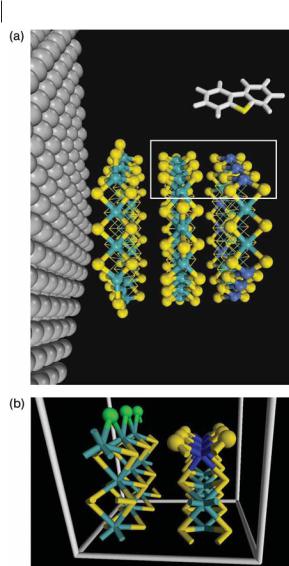
MoS2 bulk is a layered-type crystal the lattice of which is described by the hexagonal space group P63/mmc with a ¼ b ¼ 3.160 A˚ and c ¼ 12.294 A˚ [40]. Its crystal structure belongs to a family of polytypic structures with close-packed triangular double layers of S with Mo atoms arranged in the trigonal–prismatic holes of the S double layers (Fig. 9.3).

Mo atoms occupy the 2c Wyckof positions with coordinates (1/3, 2/3, 1/4) and the S atoms the 4f position with coordinates (2/3, 1/3, 0.371) [41]. Each Mo atom is bonded to six S atoms in a trigonal–prismatic arrangement. The closest SaS distances are across the double layer and within the close-packed layers; the interlayer SaS distances are much larger and of the van der Waals type. The morphology of the catalysts [16] can be depicted as small MoS2 particles (crystallites) dispersed at the surface of the support (usually SiO2, graphite, etc). These particles have an average size of approximately 600 G200 A˚ 2 and their reactivity depends on preferential exposed faces or planes. HDS catalysis is largely a surface process and, therefore, we must consider surface models. These models are usually obtained by cutting the three-dimensional bulk structure along a particular plane defined by using the appropriate Miller index [29, 39, 42]. For example, the so called basal plane of a MoS2 crystallite [36] is produced by cleaving the crystal along the (001) plane (Figs. 9.3b and 9.3c). This plane is fully covered by sulfur atoms and is inactive for HDS reactions. Cleavage of the bulk structure parallel to (010) plane (Figs. 9.3d and 9.3e) produces the well known edge surface exposing coordinatively unsaturated molybdenum or sulfur atoms. Each of the exposed Mo atoms is coordinated to four sulfur atoms and each terminal sulfur atom is coordinated to two Mo atoms. Several studies have shown that the bare Mo edge terminating in a row of undercoordinated Mo atoms is very unfavorable; such edges will therefore have high a nity for S adsorption. The real morphology of the MoS2 catalyst active sites has been deduced from experimental and theoretical studies. STM enables direct imaging of catalytically relevant surface structure on the atomic scale. By studying a realistic HDS model system consisting of a few-nanometer-wide gold-supported MoS2 particles it has been shown that the morphology of the nanoparticles is sensitive to sulfiding and reaction conditions [36]; this means triangles are formed under heavy sulfiding conditions and truncated hexagons under more sulfo-reductive conditions resembling HDS conditions. These hexagonal clusters expose the basal plane and two di erent

238 9 Atoms in Molecules Theory for Exploring the Nature of the Active Sites on Surfaces

9.3 An Application to Nanocatalyts 239

types of edge – Mo edges covered with S monomers and fully saturated S edges [36]. Di erent models have been used to study the edge structure of MoS2 catalysts using DFT methods – cluster models including a finite number of atoms [43, 44], a single SaMoaS periodic slab [45, 46], and a larger slab model containing two SaMoaS sheets exposing Mo and S edges alternately [29, 38, 39, 47–54]. From these studies a clear picture of the MoS2 edge structures has emerged. The most external Mo atoms of the Mo edge contain 50% sulfur coverage with each sulfur atom bridged to two neighboring molybdenum atoms. Significant reconstruction of the Mo edge occurs; the bridged S atoms are shifted by half a lattice constant relative to the bulk S lattice and move down to a bridging position inplane with the Mo lattice. The S edges remain fully sulfided and a maximum Mo coordination to six sulfur atoms is achieved in one configuration where the edge is terminated by a row of sulfur atoms positioned in a bridge position close to those expected from bulk-terminated MoS2. Both edge geometries lead to a coordination number of six for the outermost molybdenum atoms and two for the corresponding sulfur atoms. The local atomic structure of NiMoS catalysts has been resolved by means of DFT calculations coupled with simple thermodynamics determinations [29, 38]. Under typical sulfidation conditions nickel is preferentially incorporated into the metal edge in a square planar geometry with 0% sulfur. On a partially promoted metal edge, sulfur atoms bond to the outermost Mo atoms and the promoter atoms tend to be uncovered [38]. High-resolution electron microscopic studies of silica-supported Mo based catalysts have shown that the morphology of the catalyst can be depicted as small particles with an average size of 29 A˚ (mean diameter) and three slabs in width dispersed on the surface of the support [16]. Figure 9.4a shows a model of such a particle interacting with a dibenzothiophene molecule. The structure of the particle edge (the active site) is emphasized by means of a white square.

In this section we will study the larger periodic slab model (Fig. 9.4b) that exposes alternating layers of Mo and S edges denoting nanoparticles several layers wide. The unit cell (9:480 12:294 36:000 A˚ 3) of this surface has three and six bridged S atoms above the Mo and S edges, respectively. This cell contains a periodic slab of several layers of atoms initially having the same structure of the surface built directly from the bulk. Vacuum layers thicker than 15 A˚ were used to ensure there were no interactions between adjacent slabs. The geometry of the models was optimized by using algorithms included in the Dmol3 program [55, 56]. The two upper rows were allowed to relax while the atoms of the lower rows were kept fixed at their optimized bulk positions to simulate bulk constraints.

________________________________________________________________________________

H

Fig. 9.3 (a) Ball-and-cylinder model of the MoS2 bulk 1 2 cell illustrating the sheet arrangement of Mo and sulfur atoms.

(b) Side view of three sheets and (c) Top view of a 4 5 cell of the (001) MoS2 surface

(the basal plane). (d) Side view and (e) top

view of a 4 2 cell of the hypothetical (010) MoS2 surface. White cylinders denote the unit cell whereas light blue and yellow spheres denote the Mo and S atoms, respectively. Spheres in (e) emphasize the outermost atoms of the surface.

240 9 Atoms in Molecules Theory for Exploring the Nature of the Active Sites on Surfaces

Fig. 9.4 (a) Ball-and-cylinder model showing a side view of a hypothetical NiMoS nanoparticle that simulates the particles of

Ref. [16] supported on an Au (111) surface. Blue, dark blue, and yellow spheres denote the Mo, Ni, and S atoms, respectively, on the edges. A white rectangle emphasizes the structure of the active site that interacts with

a dibenzothiophene (white and yellow cylinders) molecule. (b) Side view of the periodic model of the MoS2 edges. Light blue and yellow cylinders denote the Mo and S atoms, respectively. Dark blue cylinders denote the Mo atoms on the S edges. Green and yellow spheres denote the outermost S atoms on the Mo and S edges, respectively.

9.3 An Application to Nanocatalyts 241

9.3.2

The Full r(r) Topology of the MoS2 Bulk

In the MoS2 unit cell, six sulfur atoms locally coordinate with one Mo atom to form a trigonal prismatic structure. Each Mo atom is surrounded by the six nearest sulfur atoms at a distance of 2.404 A˚ forming an MoS2 sheet, and each S atom is surrounded by the three nearest Mo atoms on the sheet and by the three second nearest S atoms located on a neighboring MoS2 sheet. All the CPs of that unit cell have been located and the data that characterize them are given in Table 9.2. In this table the corresponding Wycko letter in the International Tables of Crystallography [57] identifies the critical points within a unit cell. This identification is useful for determining the topology of the electron density of an extended system. Figure 9.5a illustrates the bond and cage CPS determined inside the MoS2 sheets. The bond paths are shown as gray lines connecting the bound atoms. There are six nuclei in the primitive cell, two molybdenum (light blue spheres), located at the position labeled c, and four sulfur (yellow spheres), at position f. There are twelve MoaS bond critical points (gray spheres) at position k, six four-membered ring CPs at f , and one trigonal prism-like cage (red spheres) at b.

Table 9.2	Topological properties (au) of r(r) at the critical points for
MoS2 bulk space group: P63/mmc (D4 in Schoenflies notation).
		6h
Wycko	Site	Critical point	l1	l2	l3	rb
letter	symmetry
k 12	CS	MoaS b	0.1073	0.0809	0.3212	0.0908
g 6	C2h	SaS b	0.0056	0.0056	0.0388	0.0112
h 6	C2v	Four-membered	0.0347	0.0058	0.0492	0.0433
		2Moa2S r
b 2	D3h	Three-membered	0.0149	0.0288	0.0292	0.0159
		3 Mo r
k 12	CS	Four-membered	0.0024	0.0062	0.0127	0.0070
		1Moa3S r
d 2	D3h	Red c (Fig. 9.6b)	0.0253	0.0260	0.0664	0.0311
f 4	C3v	Green c (Fig. 9.6c)	0.0048	0.0062	0.0062	0.0057
a 2	D3d	Pink c (Fig. 9.6e)	0.0017	0.0022	0.0022	0.0045
c 2	D3h	Mo n
f 4	C3v	S n