Chen The electron capture detector

DIATOMIC MOLECULES

197

Figure 9.3 Bond energies of the homonuclear diatomic anions divided by bond energies of the neutral versus atomic number. The values for the 3d elements are taken from [4]. The 4d and 5d elements are estimated to be the same as for the 3d elements.

data support the experimental and theoretical electron affinities and provide targets for the 4d and 5d elements.

9.2.2 Electron Affinities and Morse Potential Energy Curves: Group VII Diatomic Molecules and Anions

In 1985 we began a series of papers devoted to Morse potential energy curves for the halogen anions, X2( ), the rare gas positive-ion dimers, Rg2(þ), and the Group VI homonuclear diatomic anions. These curves were updated periodically based on new experimental data [8–11]. Curves for the anions of the alkali metal dimers and coinage metals dimers, M2( ), have been constructed but not published. Originally, the ground-state electron affinities for the X2 were available from gas phase experiments. The ECD had been used to measure the activation energies for thermal electron attachment. The electron impact ion distributions had been measured for all the X2 except for I2. For some of the anions the frequencies had been measured in the solid state and the absorption spectra in solution.

As early as the 1960s D. R. Herschbach calculated six Morse curves for I2( ). The data used to calculate these curves were described as follows:

Electron impact experiments only show that that the curves for some states of X2( ) must cross the ground state of the parent near its minimum. . . . The dissociation energy of I2( ) should be one half of the neutral or 0.7 eV (this gives an Ea of

198 DIATOMIC AND TRIATOMIC MOLECULES AND SULFUR FLUORIDES

Figure 9.4 Historical Morse potential energy curves for I2 and I2( ): 1966 [12] and 1985 [8].

2.3 0.5 eV). The VEa of I2 is 1.7 0.5 eV and 1.1 0.5 eV for Br2. . . . The location of the excited state curves above the minimum for the ground state has been derived from a study of color centers in doped alkali halide crystals. . . . Flash photolysis of aqueous and ethanoic solutions of alkali halides gives rise to spectra that have been assigned to the X2( ). [12]

These curves were the prototypes for the original HIMPEC classifications.

In 1985 six curves for all the X2 were obtained from updated data and ECD E1. No electron impact data existed for the two highest I2( ) curves. The original Herschbach curves and curves obtained in 1985 are compared in Figure 9.4. The

normal plot versus internuclear distance	r is replaced by a plot of	U versus
S ¼ 1 ½r=re&. R. G. Parr suggested this	variable as a technique for	spreading

out the curves in the region of the experimental data [13]. The VEa, absorption energies, activation energies, and crossings are more easily visualized with the S variable. The absorbance data used in 1985 are the same as those used in 1966. The major difference in the 1985 curves resulted from the assumed electron impact distribution for I2. The Herschbach curves are closer to the present-day curves, except that 6 curves are drawn instead of 12 [8, 12].

Figure 9.5 gives the original absorbance data used by Herschbach to draw the I2( ) curves. The energies represented by dotted lines in the 1966 data were approximated. Figure 9.6 offers the most recent data. These data are important for constructing the excited-state curves. However, before we are able to use these data, good curves for the ground-state anion must be available.

In Table 9.1 the optimum Morse parameters for the ground states of X2( ) are compared with the 1985 values, AMB and PES and theoretical calculations

DIATOMIC MOLECULES

199

Figure 9.5 Historical absorbance data for the construction of the Morse potential energy curves for the Halogen diatomic anions. The energies indicated by dotted lines were predicted in 1966 [12].

Figure 9.6 Recent absorbance data for the construction of the Morse potential energy curves for the Halogen diatomic anions. The calculated energies agree with the experimental values when available and predict experimental values which have not been measured.

200 DIATOMIC AND TRIATOMIC MOLECULES AND SULFUR FLUORIDES

TABLE 9.1 Morse Parameters for Ground State X2ð Þ

	D0 (eV)	re (pm)	n (cm 1)	AEa (eV)	References
F2( )	1.28(5)	181(5)	525(30)	3.08(5)	[5]
	1.23	192	462	3.0	[10]
	1.21(10)	179(2)	580(30)	3.08	[14]
	—	189	510	3.08	[1]
Cl2( )	1.32(2)	256(5)	255(4)	2.45(2)	[5]
	1.35	262	249	2.46	[10]
	1.30(15)	255(9)	2.4	—	[14]
Br2( )	1.18(2)	283(5)	160(4)	2.56(2)	[5]
	1.20	285	158	2.57	[10]
	1.15(10)	—	160(5)	2.6	[14]
I2( )	1.01(1)	321(0.5)	110(2)	2.52(1)	[5]
	1.01(1)	321(0.5)	111(2)	2.52(1)	[5]
	1.07	323	113	2.57	[10]
	1.02(5)	—	109	2.55	[14]
	1.01(1)	321(.5)	110(2)	—	[15]

available in the literature that best agree with experiment. The best I2( ) values derive from PES. The internuclear distances for Cl2( ) and Br2( ) are determined from the experimental VEa. The dissociation energies are defined from the AEa and Rg2(þ) values. The frequencies are experimental values measured in solids. Five or six data points define these curves, and systematic uncertainties should be smaller than random uncertainties. The parameters for F2 are less certain. The dissociation energy from the experimental AEa is 3 meV lower than the value for Ne2(þ). The internuclear distance is higher than the one obtained via AMB, but less than the NIST value. The frequency chosen is the NIST value with AMB random uncertainty. There are no ECD data for F2, but other studies give a low E1, as will be shown in simulated ECD data [1–3, 5, 8, 9, 14–19].

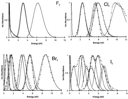
The majority of excited-state curves used the dissociation energy of the excited states of Rg2(þ) [9, 16–23]. The parameters and data used to calculate these curves are given in Table 9.2. The lower bond dissociation energy observed in the PES of I2( ) is used to calculated the 2 g1=2 curves for I2( ) [7]. By analogy two new curves for Br2( ) are calculated. Figure 9.7 presents the calculated and experimental distributions. Their agreement with experiment is apparent [20–23]. The highest curve for Cl2( ) shows two states, one of which could be for an ion pair state. The curves were then adjusted to fit the measured absorption maxima indicated in bold in Table 9.2. Four curves for I2( ) were adjusted to a common absorption maximum at 1.68 eV, as shown in Table 9.2. No attempt was made to fit the absorption distributions. The calculated values agree with experiment within the uncertainties. Each of these curves can have four points: the dissociation energy, absorbance maxima, electron impact maxima, and electron impact distribution. Some absorbance maxima are estimated by the systematic variation shown in Figure 9.6 and predicted

DIATOMIC MOLECULES

201

TABLE 9.2 Morse Parameters and Dimensionless Constants for the Neutral and Anion Morse Potentials for X2

Species						kA	kB	kR	Do	re	n 1	VEa		E(abs)
									(eV)	(pm)	(cm )	(eV)		(eV)
F2				Neutral		1.00	1.00	1.00	1.60	141	917		—	—
				2	u
F2(		)		A 2	þ	1.634	0.625	3.372	1.28	180	510		1.62	—
				B g3=2		0.555	0.525	2.840	0.170	245	159		1.07	1.67
				B 2 g1=2		0.390	0.581	2.439	0.095	247	133		0.95	1.67
				C 2 u3=2		0.379	0.390	3.692	0.060	337	71		3.06	2.88
				C 2 u1=2		0.517	0.380	4.011	0.105	322	90		3.14	2.86
				D 2 gþ		0.430	0.460	5.596	0.050	328	76.8		6.05	3.63
Cl2				Neutral		1.00	1.00	1.00	2.48	199	560		—	—
				2	u
Cl2(			)	A 2	þ	1.082	0.641	2.328	1.31	256	255		1.01	—
				B g3=2		0.431	0.638	2.370	0.191	331	101		2.66	1.64
				B 2 g1=2		0.251	0.780	2.016	0.074	331	78		2.67	1.64
				C 2 u3=2		0.324	0.655	3.251	0.077	373	67		5.41	2.35
				C 2 u1=2		0.462	0.619	3.826	0.135	368	83		6.28	2.60
				D 2 gþ		0.419	0.653	5.441	0.077	393	66	10.56		3.47
Br2				Neutral		1.00	1.00	1.00	1.98	228	323		—	—
				2	u
Br2(			)	A 2	þ	1.180	0.641	2.328	1.18	282	160		1.45	—
				B g3=2		0.438	0.598	1.926	0.195	354	61		0.70	1.32
				B 2 g1=2		0.134	0.744	1.653	0.020	400	25		1.37	1.62
				B 2 g1=2		0.147	0.728	1.671	0.024	398	27		1.35	1.62
				C 2 u3=2		0.344	0.628	3.253	0.070	410	39		3.72	2.18
				C 2 u3=2		0.383	0.632	3.546	0.080	407	42		3.72	2.24
				C 2 u1=2		0.627	0.651	4.380	0.180	380	63		5.28	2.57
				D 2 gþ		0.494	0.692	5.875	0.080	410	46		8.79	3.38
I2				Neutral		1.00	1.00	1.00	1.54	267	215		—	—
I2( )				A 1(1/2)		1.187	0.645	2.242	1.007	320.5	110	1.67		—
				A 1(1/2)		1.194	0.651	2.264	1.007	320.5	111	1.61		—
				B 1(3/2)		0.491	0.649	1.702	0.225	371	53	0.30		0.87
				B 1(3/2)		0.491	0.649	1.702	0.225	392	50		0.50	1.01
				B 1(1/2)		0.125	0.557	1.992	0.012	537	11		1.35	1.68
				B 1(1/2)		0.173	0.601	2.297	0.020	501	15		1.69	1.65
				C 1(3/2)		0.376	0.523	2.789	0.080	475	25		1.83	1.68
				C 1(3/2)		0.383	0.587	3.080	0.075	460	28		2.27	1.69
				C 2(1/2)		0.628	0.654	3.118	0.194	400	50		2.35	2.11
				C 2(1/2)		0.663	0.524	3.491	0.194	439	40		2.82	2.45
				D 2(1/2)		0.501	0.439	3.569	0.108	510	25		3.45	3.03
				D 2(1/2)		0.509	0.461	3.691	0.108	500	26		3.61	3.03

by Herschbach. The curves without these data are still defined by three points so these energies are experimental values to be compared to others.

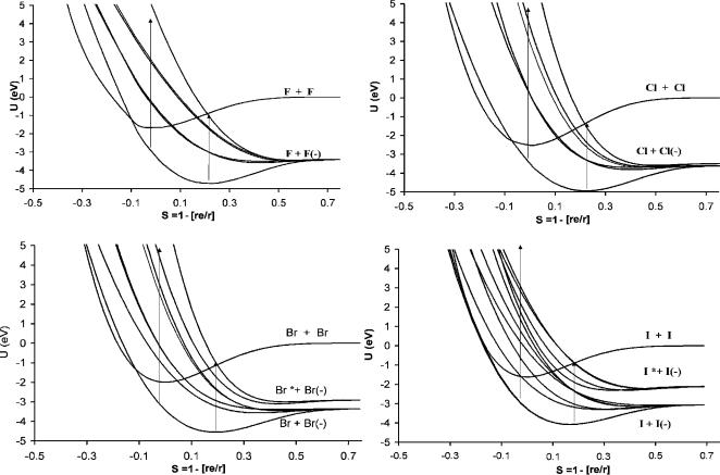
Four sets of curves are easily compared for X2, as shown in Figure 9.8. The overall similarity of the curves is striking and supports the isoelectronic principle. When we compare the values of the dimensionless constants for a given state in Table 9.2,

202 DIATOMIC AND TRIATOMIC MOLECULES AND SULFUR FLUORIDES

Figure 9.7 Experimental and calculated ion distributions for the electron impact of the halogen diatomic molecules [20–23].

this is emphasized. All the ground-state kA are greater than 1, while the kR are greater than 2. Likewise, the dimensionless constants for the D states are similar. The major differences occur in the spin orbital coupling of the atomic species. The ground-state curves are all Mcð3Þ, but the ground-state curves for F2( ) and Cl2( ) are Dð3Þ, while those for Br2( ) and I2( ) are Mð3Þ. The excited-state curves for all but the first excited state of I2( ) are Dð2Þ. The first excited state of I2( ) is Dð3Þ. The first excited-state curves for all but Cl2( ) are Mcð2Þ since they cross the neutral in the vicinity of the internuclear distance of the neutral. The remaining curves are Dð2Þ and Dcð2Þ. On the basis of this information the formation of the parent negative ions of I2( ) and Br2( ) in electron impact spectra can occur at an electron energy sufficient to overcome the activation energy for crossing to the negative-ion curve. Such ions have been observed but not explained [18, 19].

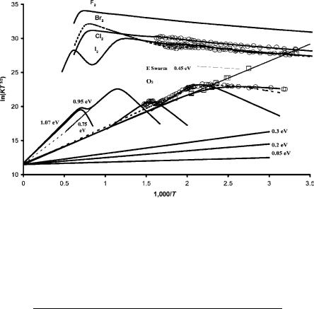
Figure 9.9 shows all the extant ECD data for homonuclear diatomic molecules [5, 10, 24, 25]. The parameters for O2 will be discussed in the next section. Originally, only one state was assumed for the halogens. If we use two states, two activation energies can be obtained from the ECD data. This requires Ea, Q, and A1 measured using other techniques or assumed. These two activation energies can be used to define two potential energy curves. The parameters utilized to calculate the ECD curves in Figure 9.9 are given in Table 9.3. The crossings of the ground

203

Figure 9.8 Morse Potential energy curves for the halogen molecules and their anions [5]. The data are given in Table 9.2.

204 DIATOMIC AND TRIATOMIC MOLECULES AND SULFUR FLUORIDES

Figure 9.9 ECD data for homonuclear diatomic molecules plotted as ln KT3/2 versus 1,000/T. The curves drawn through the data are calculated using the parameters given in Table 9.3.

TABLE 9.3 ECD Parameters for Homonuclear Diatomic

Molecules

Species	ln (A1)	E1 (eV)	Q	Ea (eV)
F2	(35.5)	(0.05)	(1)	(3.05)
F2	(33)	(0.03)	(1)	(1.7)
Cl2	(33)	0.06	(1)	(2.45)
Cl2	(35.5)	0.30	(1)	(1.1)
Br2	(35.5)	0.28	(1)	(2.56)
Br2	(33)	0.03	(1)	(1.4)
I2	(35.5)	0.45	(1)	(2.52)
I2	(33)	0.05	(1)	(1.5)
O2	(24.9)	(0.05)	(1)	(0.45)
	(24.9)	(0.05)	(0.5)	(0.43)
	(24.9)	0.1	(0.8)	(0.5)
	(34.7)	0.4	0.01	0.7
	(35.2)	0.8	0.02	0.75
	(35.5)	0.9	(0.8)	(0.95)
	(35.5)	(1.9)	(0.8)	(1.07)

The values in parentheses are experimental values from other methods or have been estimated.

DIATOMIC MOLECULES

205

state and/or the first excited states with the neutral curve agree with the E1 from ECD data. The activation energy for the backside crossing of the curves for I2( ) and Br2( ) is higher than that for the frontside crossing. Thus, dissociative thermal electron attachment will occur via the frontside curves. In the case of Cl2( ) the activation energy for the backside crossing is lower than that for the frontside crossing so dissociation occurs via the ground-state curve. These curves are prototypes for the organic halides.

9.2.3 Electron Affinities and Morse Potential Energy Curves: Group VI Diatomic Molecules and Anions

The electron affinity of the oxygen molecule is very important. In 1970 an excitedstate electron affinity for O2 was obtained from ECD data, but an unexplained upturn at higher temperatures was also present. Recent ECD results have confirmed these data, but show a second downturn at higher temperatures. These data are shown in Figure 9.9 [5, 24, 25]. Using the higher Ea from other experiments in the ECD data analysis allowed us to determine additional kinetic and thermodynamic parameters for excited states. The Ea now range from 0.15 eV to 1.07 eV: photodetachment, 0.15 (eV), 1958; CTC, 0.75, 1961 to 1971; electron swarm, 0.45, 1961; EB, 0.6, 1.1, 1961 to 1971; AMB, 0.2, 0.3, 0.5, 0.8, 1.3, 1970 to 1977; IB, 1.07, 1970; PES, 0.43, 0.45, 1971 to 1995; and ECD, 0.45, 0.5, 0.9, 0.75, 0.70, 1970 to 2002. This range is much larger than that obtained for the halogens using the same techniques, indicating significant differences [24–36]. The VEa determined from electron impact data range from 0.2 eV to 17 eV. The larger negative values are assigned to D curves [37].

In 1942 D. R. Bates and H. S. W. Massey drew potential energy curves for four bound superoxide anion states leading to O(3Pg) þ O( ) 2Pu [38]. Later 24 total

anion states were postulated: 2 g ð2Þ, 2 u ð2Þ, 4 g ð2Þ, 4 u ð2Þ, 2 þg , 2 þu , 4 þg , 4 þu ; 2 gð2Þ, 2 uð2Þ, 4 gð2Þ, 4 uð2Þ, and 2 g, 2 u, 4 g, 4 u [39]. In 1981

H. H. Michels presented curves for these states and calculated dissociation energies and Ea for the bound states of O2( ) from 1.5 eV to 3.7 eV [40]. Assigning the experimental and theoretical Ea and VEa, we obtain 12 M and 12 D HIMPEC for the 24 states [5, 41–43]. The relative bond orders of the ground state agree with simple molecular orbital predictions. The bond orders for the excited states are reasonable compared to the predicted values. Two anion curves for S2, Se2, and Te2 have been constructed from experimental data [44–47].

The experimental Ea for O2 are assigned to bound states. The VEa for these states range from 0.9 eV to 0.75 eV. The activation energies for thermal electron attachment determined from the ECD data range from 0.05 eV to 1.9 eV. The frequencies observed in solids and the Morse parameters obtained from PES, ECD, electron swarm, and other techniques can be used to approximate the internuclear distance and frequency of the predicted states. These give six Mð2Þ curves (EDEA < 0, and Ea and VEa > 0) and six Mð1Þ curves (only Ea > 0). The PES Ea, with values of 0.430, 0.450 0.002 eV, is the most precise Ea and the Born

206 DIATOMIC AND TRIATOMIC MOLECULES AND SULFUR FLUORIDES

TABLE 9.4 Electron Affinities for O2 and Morse Parameters for O2( )

States		De (eV)	re (pm)	ne (cm 1)	Ea (eV)		VEa (eV)			E1 (eV)
				Quartet States
4	u	4.6	129	1,250		0.95			0.75	0.9
4	g	4.4	130	1,210		0.75			0.5	0.8
4	gþ	4.4	130	1,210		0.75			0.5	0.8
4	u	3.9	138	1,000		0.25	0.4			0.2
4	g
4	þ	3.8	136	1,089		0.15			0.45	0.2
4	u	3.7	140	1,089		0.05	0.9			0.5
	u	1	169	700		2.65			9.5	3.5
4
4	g	0.8	183	510	2.85		9.5			3.5
	g	0.8	170	650		2.85			9.6	3.5
4	þ
4	u	0.3	220	260	3.35		10.8			4
	g	0.1	220	190		3.55		10.9		4
4	þ
	u	0.1	230	180	3.55		11.9			4
				Doublet States
2	g	4.7	129	1,250		1.07			0.86	1.9
2	g	4.35	130	1,200		0.7			0.46	0.8
2	uþ	4.15	132	1,125		0.5			0.17	0.1
2	u(1/2)	4.1	134	1,125		0.45	0.03			0.05
2
	uð3=2Þ	4.1	134	1,125		0.43	0.03			0.05
	g
2	þ	4.05	135	1,089		0.36			0.16	0.1
2	u
2		3.85	136	1,089		0.3			0.39	0.2
2	g	1.0	169	670	2.65		8.16			3
2	u	0.9	169	620	2.75		7.65			3
	u	0.82	169	610		2.82			7.77	3
2	þ
	u	0.77	169	592	2.88		7.55			3
	g	0.3	230	235		3.35		10.7		4
2	þ
	u	0.2	250	180		3.15		11.1		4
2

Haber cycle Ea at 0.9 0.1 eV is the least precise [19, 32]. The ECD values have no greater uncertainties since a data reduction procedure cannot degrade quality.

Michels calculated dissociation energies for O2( ) ranging from 0 to 2.11 eV for nine bound states. These give negative Ea and VEa but dissociate in the Franck Condon region. Therefore, they are all Dð0Þ curves. The only M curve presented was determined from PES data with an Ea of 0.45 eV [31]. Between the ground state and first excited 2 u state there are three quartet states and two doublet states separated by 1 eV. By assigning the experimental values to the predicted order, the Ea shown in Table 9.4 were obtained. The Ea of the 4 u state is assigned to 0.95 eV, and the electron affinities of the 4 g state and accidentally degenerate 4 þg state are assigned Ea ¼ 0:75 eV. The next two doublet states are assigned these Ea: 0.7 eV and 0.5 eV [28–30]. The five other bound states are assigned Ea of 0.4, 0.3, 0.25, 0.15, and 0.05 eV, yielding 12 states with positive Ea that lead to molecular anions, 6 Mð2Þ and 6 Mð1Þ states [5, 26, 31–36].