Chen The electron capture detector

STRUCTURES OF ORGANIC MOLECULES

337

Structure 1 (Continued)

Adiabatic Electron Affinities, Gas Phase Acidities, and Names of the DNA and RNA Bases

Structure 2

338 APPENDIX II

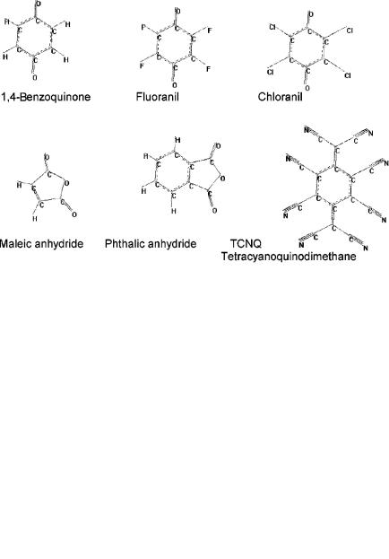
Charge Transfer Complex Acceptors

Structure 3

Aromatic Hydrocarbons and Numbering System

Structure 4

APPENDIX III

General Least Squares

Any hesitancy to use statistical analysis has probably stemmed from the time-consuming and tedious calculations. This is especially true in least squares where the function relating the variables is complicated and may involve multiple parameters to be determined from variables which have comparable errors. . . . With the advent of high speed computers, the difficulty in this task can be eliminated.

— W. E. Wentworth

Journal of Chemical Education

Here examples of least-squares adjustments of experimental data will be presented. For measurements with equal uncertainties the average is the least-squares ‘‘best’’ estimate. For a series of measurements with unequal uncertainties the values should be weighted according to their uncertainty. This was discussed for the determination of the current ‘‘best’’ value for the Ea of bromine. The adjustment for a linear two-parameter equation with equal errors in only one direction, as is generally carried out in trendline programs, is compared to the adjustment of data with unequal errors in both the X and Y. The determination of experimental electron affinities from ln KT3=2 versus 1,000/T for acetophenone is an example of this type of adjustment. The unequal weights result because the original data, K and T, are transformed into a linear equation.

Next we consider the general problem, where the variables x, y, z, . . . and parameters a, b, c, . . . are related by a mathematical relationship obtained from fundamental principles. That is, there is a fundamental function F(x, y, z, . . . ; a, b, c,. . .) ¼ 0. An example is the extended equations for ln KT3=2 versus 1,000/T, where the variables are K and T, and the parameters are the pre-exponential and energy quantities for the rate constants of attachment, detachment, and dissociation for the ground and excited states. There can be as many as eight parameters and two variables. The experimental variables and errors in each of the sx and sy variables must be estimated. The parameters a, b, . . . and errors in parameters, sa, sb, . . . , result from the adjustment procedure. In addition, the covariance terms sab and sac are obtained. These are used in the propagation of error in other quantities.

339

340 APPENDIX III

First, it is necessary to describe the general principle of least squares and to define the symbols that will be used in the examples. For this, we will return to Deming:

In all adjustments of observations, simple or complicated, the principle of least squares requires the minimization of the sum of the weighted squares of the residuals. This sum may be written

S ¼ Sum ¼ wðresÞ2 ¼ fwx Vx2 þ wyVy2g

AIII:0

S is called the sum of the weighted squares.

The weights are proportional to the reciprocal of the errors squared in the experimental values. The quantity Vx and Vy are the x and y residuals. The principle of least squares is the minimization of S. The method of least squares is a rule or set of rules for proceeding with the actual computation. [Chap 4, 36, p. ?]

If the errors in the experimental parameters can be estimated or are known for a given experimental measurement, then the errors obtained in parameters from a specific experiment can be compared with these values and the quality of the results from a specific experiment evaluated. The ‘‘known’’ errors are designated s(o). In the statistical treatment of data this is designated as the ‘‘true’’ standard deviation, while the standard deviation from a given experiment is designated with the symbol s or s(ext).

The standard formulation of least-squares adjustments of a linear equation can be solved in a closed form and the errors in the parameters calculated directly. This formulation is often given as an example of the use of partial differential calculus in a practical situation. If the errors are equal and exist primarily in the y variable, the mathematical function to be minimized is

½F2ðx; y; a; bÞ& ¼ ðyi a bxiÞ2

ðAIII:1Þ

The derivative of F with respect to a and to zero, where Fðx; y; a; bÞ ¼ y a bx,

b (Fa and Fb) is then taken and set equal to give

Fa ¼ 2 ðyi	a	bxiÞð	1Þ ¼ 0	ðAIII:2Þ
Fb ¼ 2 ðyi	a	bxiÞð	xiÞ ¼ 0	ðAIII:3Þ

These can be solved directly for a and b and their errors. This is the procedure that is used in standard trendlines. The problem with this procedure is that the random errors only occur in the y variable and the errors are assumed to be equal. In many cases there are unequal errors in both variables.

We define the summations as ½y& ¼ yi½x& ¼ xi; ½xy& ¼ xyi; ½xx& ¼ x2i n ¼1. Then

na þ b½x& ¼ ½y&		and a½x& þ b½xx& ¼ ½xy&	ðAIII:4Þ
and using Cramer’s rule, we obtain
a ¼ ð½y&½xx& ½x&½xy&=D;	b ¼ n½xy&	½x&½y&=D; D ¼ n½xx& ½x&½x&	ðAIII:5Þ
sa2 ¼ f½F2ðx; y; a; bÞ&=ðn	2Þg½xx&=D;	sb2 ¼ f½F2ðx; y; a; bÞ&=ðn 2Þgn=D	ðAIII:6Þ

GENERAL LEAST SQUARES

341

Thus, by simply calculating [x], [y], [xx], [xy], and [F2ðx; y; a; bÞ], the quantities in equations AIII.5 and AIII.6 can be obtained.

Figure AIII.1 is an example of the fit for ln KT3=2 ¼ Y ¼ aest þ best X. The errors are all assumed to fall in the Y direction. The values of the parameters are aest ¼ 12.37(7) and best ¼ 3,572(138). This gives an Ea of 0.310(14) eV and a Qan

3=2	A linear least-squares fit to the function Y	¼	aest	þ	best X, where Y is
Figure AIII.1

ln(KT ) and X is 1/T for acetophenone at a reaction time of 50 ms. The plot is the trendline that shows the equivalence of the trendline and the normal least squares.

342 APPENDIX III

of 2.00(10). Both of these are different from the ‘‘best’’ values of 0.338(2) eV and 1.00(5).

Other problems with this simple approach are that estimates of the parameters obtained from other experiments or which are indicated by theory cannot be included in the adjustment. For example, if the intercept has been determined by a series of other experiments to be a sa, it is appropriate to include that value in the adjustment of new data to estimate the slope b. Alternatively, if the slope b is 1:0 0:05, then this should be included in the adjustment to obtain a more precise value of a. Also, the quality of the fit of the data to the function is often not realistic because of the assumptions concerning the random errors. Finally, it is difficult to consider additional variables and/or parameters or nonlinear functions. Thus, the use of a general least-squares operation is possibly more valuable than this simple approach and with modern spreadsheets is no more difficult.

The general treatment of least squares presented by Deming eliminates these problems and is not much more complicated than the closed form of the equations given above. In addition, the transformation of a nonlinear equation to a linear one can be accomplished quite simply with the proper weights. We will not present a derivation of the procedure since it has been described previously. We will simply present examples of the steps in the procedure for a two-parameter case. The extension to more than two variables is simple since there is no increase in the size of the matrix to be inverted. The extension to more than two parameters does involve an increase in the size of the matrix but is apparent.

The exact solution of the minimization equations obtained from AIII.2 is not usually attempted. Rather, an ‘‘iterative’’ method is used. Reasonable approximations or ‘‘guesses’’ of the parameters are made and improvements to the guesses are calculated. As long as the guesses are relatively good, the procedure will ‘‘converge’’ so that the changes in the guesses are small and the value of S is a minimum. With a macro and a modern spreadsheet such as EXCEL, the repeated application of this procedure will result in convergence within a short period of time. The eventual result is the ‘‘best’’ values of the parameters consistent with the experimental data and, more significantly, estimates of the errors as given by the variances and covariances of the parameters so that other quantities can be calculated from ‘‘new’’ data.

Wentworth summarized these advantages as follows:

Of primary importance are the estimates of the errors of the parameters which may be used directly in interpreting or evaluating the parameters or in the propagation of errors upon the calculation of subsequent quantities. The actual parameters should be the most probable values if the errors are truly random, following a Gaussian distribution. From the experimental data and the associated errors, an experimental apparatus (procedure) can be pre-evaluated in regards to the desired accuracy of the results. If the errors of the observations are well characterized, a statistical test can be applied to evaluate how well the data fit a given function. This can aid the investigator in deciding whether a theoretical or empirical function of the variables is satisfactory and whether a further critical evaluation of the theoretical function is justified.

Other advantages are that it is possible to include estimates of parameters and their errors in the adjustment procedure to obtain more precise values of unmeasured

GENERAL LEAST SQUARES

343

parameters. The procedures can be carried out rapidly using modern desktop computers. The calculation procedure is no more complicated than for the closed solution form.

The first step in the procedure is to assemble the data xi, yi, sxi, and syi. These are entered in columns on the spreadsheet. Then the expression for the function is written in terms of the variables and parameters, for example, F1, F1 ¼ y a bx, or

F2 ¼ lnðKT3=2Þ a	b=T. The next step is to find the derivatives F0x, F0y, F0a,
and F0b:
F10x ¼ b;	F10y ¼ 1; F10a ¼ 1;	F10b ¼ x
F20T ¼ f1=ðKT3=2Þgfð3=2ÞT1=2g þ b=T2;		F20K ¼ 1=ðKT3=2Þ;
F20a ¼ 1;	F20b ¼ 1=T

The analytical expressions for these derivatives are then entered into the spreadsheet. Subsequently, the term Li ¼ ðF0xÞ2ðsxÞ2 þ ðF0y2ÞðsyÞ2 is calculated in a separate column. Next a and b are estimated. These are defined as aest and best. Then the function is calculated in a separate column using these estimates; it is designated F0. Next the quantities F0aF0a=L, F0bF0b=L; F0aF0b=L; F0F0=L; F0aF0=L; and F0bF0=L are calculated and the sums over the data points taken. These sums are used in a matrix to calculate the corrections to the estimated parameters. New estimates are then calculated and the procedure carried out until the changes in the parameters are small.

The equations to be solved can be written as

½a0a0& a þ ½a0b0& b ¼ ½F0a0& and ½a0b0& a þ ½b0b& b ¼ ½F0b0&

where the brackets indicate sums and the term a0a0 is Fa0Fa0=L, etc. In matrix form this is

	a0a0	a0b i		a					F00 a	&
	½a0b0& ½b0b&0			b		¼		½F0
	½	& ½ &						½	0b	&

This equation can be solved by Cramers’ rule as above or by finding the inverse matrix.

In many spreadsheets there is a matrix solution routine that will carry out this procedure. Such is convenient for larger matrices. For example, for the leastsquares solutions for two negative-ion states for ECD data, there are eight parameters to be determined. The elements of the inverse matrix are designated as d’s.

The corresponding table is

X sX Y sY x0	y0	L a0	b0	F0	F0F0	a0a0	a0b0	b0b0	F00 a	F00 b
--- --- --- --- ---	---	--- ---	---	---	---	---	---	---	---	---
					---	---	---	---	---	---
					-----	-----	-----	-----	-----	-----
					½F0F0&	½a0a0&	½a0b0&	½b0b0&	½F00 a&	½F00 b&
					g0	g1	g2	g3	g4	g5

344 APPENDIX III

These calculations can be completed using the spreadsheet functions. The iteration is controlled using a Visual Basic MACRO. The inverse matrix gives the errors and covariances. The errors in the parameters will be obtained from the inverse matrix. They are ðsaÞ2 ¼ daa S, where S is [F0F0]/(n 2) for the two parameters that are

determined from the data. Likewise, ðsbÞ2 ¼ dbb S and sab, the covariance term, is dab S.

With more than two variables the L terms are simply expanded to include more terms. For a two-parameter equation the size of the matrix remains 2. For a sixparameter equation with two variables, the size of the matrix is a symmetrical 6 6. Thus, only 27 sums need be calculated. The 6 6 square matrix is inverted and multiplied by the 1 6 matrix to obtain corrections in the six parameters. These are then adjusted and the process iterated to convergence. The iteration is controlled with a Visual Basic Macro. The rigorous inclusion of estimates for parameters from other experiments is easily incorporated into this procedure. The parameters and errors must be input. Next the program simply adds terms to the appropriate sums. For example, if the value of a has been determined to be ax with an uncertainty of sa, then the quantity 1=ðsa saÞ is added to [a0a0] and this quantity is multiplied by (aest ax) and added to [F0a0]. The adjustment is made as before, as are the parameters and uncertainties obtained. This has been demonstrated by Wentworth, Hirsch, and Chen [Chapt. 5, 37].

The calculation of another quantity from the parameters and their errors can then be carried out. If a property p ¼ a þ ða þ bÞ=b3 has some physical significance, then the error in P may be calculated using the propagation of error as

S2p ¼ p2as2a þ p2bs2p þ 2papbsab

¼ ð1 þ 1=b3Þ2s2a þ fða=b3Þ 3ða þ bÞ=b2g2s2b þ 2ð1 þ 1=b3Þfða=b3Þ 3ða þ bÞ=b2gsab

In the majority of presentations the last term, the covariance term, is not included. However, it can be a very important portion of the error in the calculated quantity. The general least-squares procedure calculates this quantity as indicated above.

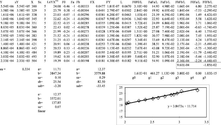
An example of the calculation for F2 ¼ ln KT3=2 aest best(1,000/T) is shown in Figure AIII.2. The derivatives are given above. Only five sums should be taken, but the equations must be iterated to minimize the function. In Figure AIII.2 the parameters from the program with equal errors in T and a constant fractional error of 10% in K give essentially the same results as a linear least squares. The values of the parameters are aest ¼ 12.37(29) and best ¼ 3,572(83).

If the ‘‘known’’ Ea of 0.338(2) eV is used in the data analysis by adding 1/ (sa sa) to the [a0a0] term and this quantity is multiplied by (aest ax) and applied to [F0a0], a rigorous least-squares solution can be obtained, as shown in Figure AIII.3. The added terms were originally zero. The intercept is 11.71(10) and the slope 3,847(26). This gives an Ea of 0.334(3) eV and a Qan of 1.00(1).

345

Figure AIII.2 Nonlinear least squares with equal weights in the temperature and equal fractional errors in K. The parameters are slightly different from the simple linear least-squares solution and the variances and covariances are calculated.

346

Figure AIII.3 The weighted average value for the slope is included in this data reduction with its uncertainties. This simply requires the addition of two terms to the sums, g4 and g5. If estimates exist for both the slope and intercept, these can be added to the data to obtain the rigorous solution and uncertainties.