Physics of biomolecules and cells

158 Physics of Bio-Molecules and Cells

length and barrier width are tied to curvatures (κ = ∂2E/∂x2) of the energy

landscape at the

minimum and transition states, i.e. L

c

≈ (2πkBT /κc)

1/2

1/2

and Lts ≈ (2πkBT /κts)

respectively. (Note: These approximations fol-

low2 from expansions

of

energies to

quadratic order, E

−

E

κ

(x

−

2

0 ≈

c

x0) /2, and, E − Eb

≈ −κts(x − xb)

/2, in the vicinity of the minimum

and transition state respectively.) We now have Kramers’ classic prescription [16, 18] for attempt frequency in an overdamped liquid environment, i.e. D/LcLts = (κcκts)1/2/2πζ, and the corresponding di usive relaxation time tD = 2πζ/(κcκts)1/2. Although little is known about these molecularscale properties, damping coe cients of 2−5 × 10−8 pN-sec/nm are typically deduced from molecular dynamics MD simulations of bonds under force [15, 17, 22]. Assuming a product of length scales LcLts on order of 0.01–0.1 nm2, Kramers theory predicts that kinetics are driven by an attempt frequency of 1010−109/s, but actual rates of dissociation end up at1/s for barrier heights of 21kBT , or, astonishingly, at 1/40 years for barrier heights of 42kBT , and so on!

1.3 Link between force – time – and bond chemistry

1.3.1 Dissociation of a simple bond under force

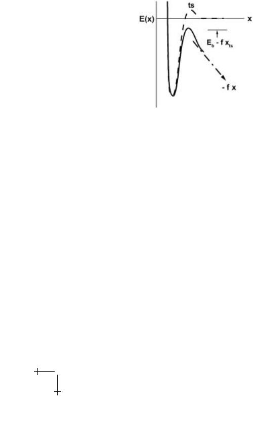
As illustrated in Figure 1.6, application of a persistent-external force (independent of distance) to a bond contributes a mechanical disjoining potential that deforms the chemical energy landscape. Energy barriers are lowered, displaced inward, and narrowed in ways that significantly a ect kinetics. The shapes, levels, and locations of intervening minima are also altered but as we’ll see, this has little impact on rate of dissociation provided that there is no switch in location of the primary minimum. Neglecting many subtle features, shifts in locations and changes in widths of barriers merely introduce weak prefactor dependencies on applied force in the unbonding rate (e.g. 1/Lts f α with α 1 or less, see Ref. [10]), which become insignificant for sharp energy barriers and so will be suppressed here. The major impact on kinetics stems from the enormous increase in likelihood of unbonding as barriers fall under applied force.

Force lowers a barrier in proportion to its thermally-averaged projection xβ = xts cos θβ along the pulling direction, i.e. Eb(f ) = Eb −f xβ ; the angle θβ accounts for instantaneous deviations of the reaction coordinate from this direction. The reduction in energy under force leads to exponentiation

of the rate of barrier passage, i.e. ν→∞ = (1/tD)exp(−Eb/kBT )exp(f xβ/kBT ), as first hypothesized by Bell [4] over twenty years ago. Consequently, the

characteristic scale for force is determined by thermal activation, i.e. fβ = kBT /xβ , which can be surprisingly small since kBT ≈ 4.1 pN nm at room temperature and xβ 0.1−1 nm. Thus, because of

E. Evans and P. Williams : Dynamic Force Spectroscopy

159

Fig. 1.6. Coupled to the projected reaction coordinate x, a persistent-external force f adds a mechanical potential – f x that tilts the landscape and lowers the barrier to dissociation. (Note: from here on, f represents an externally applied force fext.)

thermal activation, pulling on a bond with forces of a few times the thermal force fβ will cause a bond to dissociate a hundred or thousand times faster than it would spontaneously. But to break a bond in less than a nanosecond, it can take 40–50 times the thermal force fβ , as demonstrated in molecular dynamics simulations [15, 17, 21, 22].

1.3.2Dissociation of a complex bond under force: Stationary rate approximation

Since macromolecular bonds involve widely-distributed atomic-scale interactions, a rough terrain of barriers can exist in the energy landscape even after averaging over fast degrees of freedom before reaching laboratory time scales. When force is applied, outer barriers are driven below inner barriers so that an inner barrier becomes the dominant impedance to unbinding as sketched in Figure 1.7. We will see that switching of the prominent barrier leads to a hierarchy of exponential amplifications in rate of escape under force.

Unlike an ideal single-level transition, analysis of a multilevel transition under changing force is not transparent and usually requires numerical computation or simulation. However, we can develop useful approximations for the e ective rate of unbonding over a cascade of N -1 sharp barriers that separate N levels (minima). These approximations follow directly from Kramers stationary-flux theory. Step-wise integration of the flux J from

160	Physics of Bio-Molecules and Cells

Fig. 1.7. Conceptual switching of dominant energy barriers in complex bond as the outer barrier is driven below an inner barrier by application of force.

one level to the next yields coupled equations that relate the rate of complete transition ν→(= J in 1-D) to the densities of states ρn at each energy minimum Ec(n) along the energy contour. With energies defined relative to the first minimum (i.e. Ec(1) = 0), the initial integration from the first (n = 1) to second minimum (n = 2) gives,

ν→ Lts(1) exp[Ets(1)/kBT ]/D = P1/Lc(1) − P2 exp[Ec(2)/kBT ]/Lc(2) (1.10)

which is followed by integration through intermediate levels,

ν→ Lts(n) exp[Ets(n)/kBT ]/D = Pn exp[Ec(n)/kBT ]/Lc(n) . . .

− Pn+1 exp[Ec(n + 1)/kBT ]/Lc(n + 1) (1.11)

all the way to the unpopulated N th level where PN = 0 (i.e. an adsorbing state),

ν→ Lts(N − 1) exp[Ets(N − 1)/kBT ]/D =

PN −1 exp[Ec(N − 1)/kBT ]/Lc(N − 1). (1.12)

Here, the density of states ρn at each minimum is expressed in terms of the likelihood (probability) Pn of being at that level, scaled by a confinement length Lc(n) as defined earlier, i.e.

ρn = Pn /Lc(n) and Lc(n) = dx exp{[E(x) − Ec(n)]/kBT } ·

n

E. Evans and P. Williams : Dynamic Force Spectroscopy

161

Also, barrier widths Lts(n) are again introduced to represent the energyweighted integrals local to each transition state at energy Ets(n),

Lts(n) = dx exp{[E(x) − Ets(n)]/kBT } ·

n→n+1

For convenience, we idealize the landscape as a sequence of narrow minima and sharp transition states having the same confinement length Lc(n) = L0 and barrier width Lts(n) = Lb. In this way, a common relaxation time tD = L0Lb/D is defined for all transitions, and equations (1.10–1.12) predict Boltzmann-weighted likelihoods for levels, i.e.

tD ν→Σj=1→N −1{exp[Ets(N − j)/kBT ]} = P1	(1.13)
.
tD ν→Σj=1→N −n {exp[Ets(N − j)/kBT ]} = Pn exp[Ec(n)/kBT ]	(1.14)
.
tD ν→{exp[Ets(N − 1)/kBT ]} = PN −1 exp[Ec(N − 1)/kBT ].	(1.15)

At equilibrium, we expect each weighted likelihood to be unity, i.e. Pn → exp[−Ec(n)/kBT ].

However, for the non-equilibrium process of unbonding, the likelihood of being in a particular level will deviate from a Boltzmann distribution. Two particular cases provide limiting initial conditions for the distribution of states in the stationary flux model. The first limit represents a strongly bound complex where the vast majority of states lie in a deep primary minimum, i.e. P1 ≈ 1. In this case, the approximate rate of unbonding is given by equation (1.13) [7, 8],

ν→ ≈ (1/tD)/Σn=1→N −1 exp[Ets(n)/kBT ].

(1.16)

No surprise, we see that the rate of unbonding is dominated by the largest exponential, which is set by the highest transition state relative to the primary minimum. But for complexes with low-lying secondary minima, partial filling of intermediate levels may a ect the unbonding rate in ways that can become important under force. This case is easily treated using the auxiliary requirement that the occupation of inner levels add up to one, i.e. Σ1→N −1Pn = 1 (as noted by Ajdari et al. [3]). In this case, the unbonding rate is found by rearranging equations (1.13–1.15) to obtain the Pn’s and then evaluating their sum, i.e.

ν→ ≈ (1/tD)/Σn=1→N −1 exp[−Ec(n)/kBT ]Σj→N −n exp[Ets(N − j)/kBT ]. (1.17)

162	Physics of Bio-Molecules and Cells

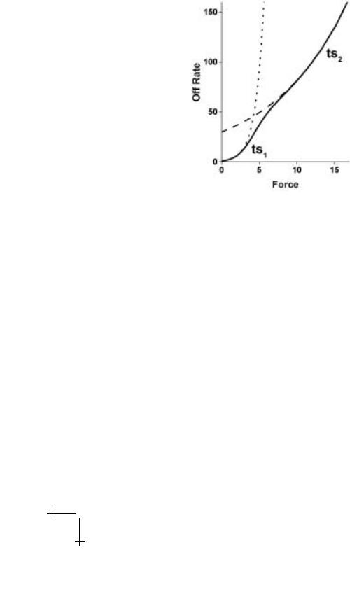
Fig. 1.8. Amplification of unbonding kinetics under persistent force for an energy landscape of two barriers as depicted in Figures 1.3 and 1.7.

As expected, the approximation in equation (1.17) reduces to equation (1.16) when metastable levels are more than a few kBT above the primary minimum.

So how does external force a ect the rate of unbonding over a multilevel energy landscape? Given narrow minima bounded by sharp barriers, the energies at these locations will change through proportionalities to force set by projections of the minima xc(n) and barriers xβ (n) along the pulling

direction, i.e. Ec(n) ≈ E0(n) − f xc(n) and Ets(n) ≈ Eb(n) − f xβ (n). This introduces exponential dependencies on force into the approximations for

unbonding rate, i.e.

ν→ ≈ (1/tD)/Σn→N −1 exp[Eb(n)/kBT ] exp[−f xβ (n)/kBT ]	(1.18)
ν→ ≈ (1/tD)/Σn=1→N −1Σj→N −n exp{[Eb(N − j) − E0(n)]/kBT }
× exp{f [xc(n) − xβ (N − j)]/kBT } ·	(1.19)

Hence, consistent with a changing hierarchy of barriers, application of force to a complex bond leads to an sequence of exponential increases in unbonding rate as illustrated in Figure 1.8.

E. Evans and P. Williams : Dynamic Force Spectroscopy

163

Table 1.1. Master equations for unbonding in an N -level system.

bound

dS1/dt = −ν1→2S1(t) + ν1←2S2(t)

.

.

dSn/dt = −{νn→n+1 + νn−1←n }Sn (t) + νn−1→n Sn−1(t) + νn←n+1Sn+1(t)

.

.

unbound

dSN /dt = −νN −1←N SN (t) + νN −1→N SN −1(t)

1.3.3 Evolution of states in complex bonds

To describe the detailed evolution of states in a complex bond, a hierarchy of “master equations” (Table 1.1) is needed to predict the likelihood Sn (t) of being in the nth level (local minimum) as a function of time. In this Markov sequence, the forward νn→n+1 and reverse transition rates νn←n+1 at each barrier depend exponentially on the height of the barrier relative to the adjacent minima. Assuming a simple 1-D topology where xc(n) < xβ (n) < xc(n + 1), forward rates of barrier passage would increase under force as,

νn→n+1 = (1/τn→n+1) exp{f [xβ (n) − xc(n)]/kBT }	(1.20)
and reverse rates would decrease as,
νn←n+1 = (1/τn←n+1) exp {−f [xc(n + 1) − xβ (n)]/kBT } ·	(1.21)

The prefactors in these expressions are the spontaneous rates of transition defined by the initial height of a barrier Eb(n) relative to its adjacent minima E0(n) and E0(n + 1),

(1/τn→n+1) = (1/tD) exp{−[Eb(n) − E0(n)]/kBT }
(1/τn←n+1) = (1/tD) exp{−[Eb(n) − E0(n + 1)]/kBT } ·	(1.22)

Even with ideal exponential dependencies of transition rates on force, these master equations can only be solved analytically when force is constant. In this case, Laplace transform of the master equations leads to a linear system of algebraic equations in transform space. This set of equations can be diagonalized and inverse transformed to obtain a superposition of decaying exponentials in time that describe the probability of reaching the unbonded state. However, as we will see next, probe tests of bonds and dynamic force spectroscopy in particular involve changing levels of force

164	Physics of Bio-Molecules and Cells

in time. Under rising force, the dynamics of multilevel transitions can be extremely complex and solution of the master equations will require numerical computation or tedious Monte-Carlo simulation. Fortunately, the strong exponential dependence on force and wide separation of energy barriers in real interactions often allow transitions from bound to free states to be described by a stationary-rate approximation (Eqs. (1.16) or (1.17)) and a single master equation. In this way, we will demonstrate that multilevel unbonding under increasing force leads to a distinct pattern of force versus loading rate, which is the basis of dynamic force spectroscopy.

1.4 Testing bond strength and the method of dynamic force spectroscopy

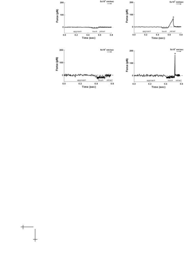
With few exceptions, tests of bond strength with force probes usually follow a common approach. The probe tip and substrate are first decorated with reactive molecules using methods that vary from nonspecific adsorption to covalent attachment with heterobifunctional polymer spacers or noncovalent attachment by high-a nity complexes such as biotin-streptavidin. Once prepared, a probe and substrate are repeatedly brought to/from contact by steady-precision movements. If decorated with a very low density of reactive sites, repeated contact between the probe tip and test surface will only result in an occasional bond. Under controlled conditions of contact, a low frequency of attachment provides quantitative verification of the likelihood of rare-single bond events (e.g. probability >0.9 when 1 attachment occurs out of 10 touches). When a bond has formed, the tip is held to the substrate and the probe transducer (“spring”) is stretched as the surfaces separate. Bond rupture is signalled by rapid recoil of the transducer to its rest position and the maximum transducer extension yields the rupture force. Histories of force over the course of approach – touch – separation with and without formation of a bond are demonstrated in Figure 1.9. After numerous touches, the few detachment forces are cumulated into a histogram (as will be shown later). The peak in this histogram is the most likely force for rupture and establishes a statistical definition for bond strength. Surprisingly, we’ll see later that no matter how carefully measured or precise the technique, bond forces will always be spread in value and the most frequent breakage force will depend on how fast force is applied to the bonds. The crucial feature of the typical probe test is that the force experienced by a bond rises in time. As seen in Figure 1.9, a bond broken under slow loading has a long lifetime but only withstands a small force; whereas, the same type of bond broken under fast loading has a very short lifetime and withstands a large force. We will see that when plotted on a logarithmic scale of loading rate (force/time), measurements of rupture force over an enormous span in rate from very slow to extremely fast image the prominent energy barriers traversed along the dissociation pathway.

E. Evans and P. Williams : Dynamic Force Spectroscopy

165

Fig. 1.9. Examples of tests performed at slow (upper plots) and fast (lower plots) speeds with a biomembrane force probe BFP (shown in Fig. 1.10). The force is traced over time in the course of approach–touch–separation with (right) and without (left) formation of a bond.

1.4.1 Probe mechanics and bond loading dynamics

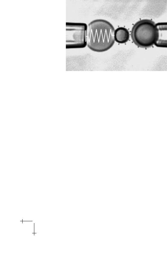
At present, measurements of single bond strength are usually performed with one of three types of apparatus: (i) the atomic force microscope AFM [5] where force is sensed by deflection of a thin silicon nitride cantilever; (ii) the biomembrane force probe BFP [11] where force is sensed by axial displacement of a glass microsphere glued to the pole of a micropipetpressurized red blood cell (example in Fig. 1.10); and (iii) the laser optical tweezer LOT [1, 2, 19, 31] where force is sensed by displacement of a microsphere trapped in a narrowly-focused beam of laser light. Each of these probes acts as a very soft spring with a small elastic sti ness κf (force ∆f per deflection ∆x) that ranges from <1 pN/nm to 1 nN/nm. Low values of probe sti ness represent high sensitivity to force for each nm deflection of the spring but also large thermal fluctuations in position (δx2 kBT /κf ). On the other hand, high probe sti ness represents low sensitivity to force per unit deflection and large thermal fluctuations in force (δf 2 kBT · κf ).

As seen in Figure 1.9, bond strength and lifetime depend critically on how fast force is applied which involves both sti ness of the spring that

166	Physics of Bio-Molecules and Cells

Fig. 1.10. Prepared to test a ligand-receptor interaction, a biomembrane force probe (symbolized by the “spring” – left) with a glass tip decorated by the ligand (“pin heads”) is shown on approach to a glass bead (right) decorated by the receptor (“darts”). The pipet suction ∆P applied to the red blood cell transducer (scaled by pipet radius Rp) sets its membrane tension τm Rp∆P and thereby tunes the elastic sti ness κf of the transducer “spring”, i.e. κf τm.

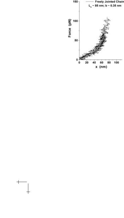
pulls on the bond and the pulling speed v. However, even with a known product of probe sti ness and separation speed, the rate of force application to a bond can deviate signficantly from this expected value when soft molecular structures connect the bond and probe. If the bond is linked symmetrically to tip and substrate by components with the same sti - ness κm, the e ective spring that pulls on the bond has a compliance given by, 1/κs = 2/κm + 1/κf . Most biomolecules are linked to solid surfaces by highly flexible polymers. These connections have a nonlinear elastic response and a very small thermal scale kBT /(Lpb) for sti ness that depends on contour length Lp and persistence length b of the polymer. Even for relatively short linkers, the sti ness scale is <1 pN/nm. So when connected to a sti probe (e.g. with κf > 10 pN/nm), the soft linker becomes the effective spring that pulls on the bond but applies a nonlinear loading history as seen in Figure 1.11. In addition, bond rupture almost always occurs in the asymptotic regime of loading as the polymer is pulled taut. Here, force diverges f ≈ (kBT /cb)/(1 − x/Lp)α as length x → Lp, with α = 1 & c = 1 for a freely-jointed polymer and α = 2 & c = 4 for a worm-like polymer. Under constant pulling speed (x = v t), loading increases rapidly with an approximate rate, rf (t) ≈ (kBT /cLpb)v/(1 − vt/Lp)α+1. We will see later

E. Evans and P. Williams : Dynamic Force Spectroscopy

167

Fig. 1.11. Loading of bonds formed between the biotinylated glass tip of a BFP and an avidinated latex microsphere (superposition of 8 tests). The plot shows that the bonds are anchored to the latex microsphere by long, flexible chains of polystyrene.

that this unsteady loading plays an important role in the dependence of rupture force on detachment speed.

What’s subtle with operation of any probe in liquids is that hydrodynamic interactions always accompany relative motion between the probe and substrate. Moreover, each hydrodynamic situation has to be analysed carefully to determine the impact on probe force. But a particularly important e ect is the hidden contribution to force ∆f that arises when a probe is pulled quickly; the force augmentation is governed by the probe damping coe cient ζ and deflection speed v, i.e. ∆f = ζv. In general, the damping coe cient is proportional to viscosity η of the liquid environment and a hydrodynamic profile length Lζ for the probe, i.e. ζ ≈ ηLζ . As such, damping coe cients are in the range from 10−5 pN-s/nm for a micron-size particle trapped by LOT to 10−4 pN-s/nm for a BFP and 10−3 pN-s/nm for a long AFM cantilever, which implies viscoelastic response times tf ζ/kf in the range of 10−5−10−3 s. Unfortunately, damping coe cients are difficult to predict accurately by theory and usually have to be measured. As an example of such measurement, Figure 1.12 shows the recovery of a BFP following release from a deflecting force at three di erent settings of elastic