Physics of biomolecules and cells

148	Physics of Bio-Molecules and Cells

demonstrate the kinetic origin of the force distribution, the peak of which defines bond strength. Finally, we show how these developments come together to establish the method of dynamic force spectroscopy and give examples of single molecule experiments. In the second chapter to follow, we describe how a nanoscale attachment made up of a few bonds fails under force and develop limiting models for use in analysis of probe tests that involve multiply-bonded contacts.

1.1.1 Intrinsic dependence of bond strength on time frame for breakage

Unlike interatomic linkages within nucleic acid – protein – lipid – carbohydrate structures, weak noncovalent bonds between these biomolecules have limited lifetimes and will dissociate under almost any level of force if pulled on for modest periods of time. When close to equilibrium in solution, large numbers of molecules continuously bond and dissociate under zero force; thus, application of a field (e.g. electrical force or osmotic stress) to the reacting molecules simply alters the ratio of bound-to-free constituents. But at infinite dilution, an isolated molecular complex (“bond”) exists far from equilibrium and has no strength on time scales longer than the time to = 1/Ko needed for spontaneous dissociation. If pulled apart faster than to , a solitary bond will resist detachment. The unbonding force can range up to – and even exceed – the adiabatic limit f∞ |∂E/∂x|max defined by the steepest gradient in the intermolecular potential E(x) that binds the complex. In other words, if the bond is broken in less time than required for di usive relaxation ( 10−9 s), the force must exceed the “brittle” fracture strength of the bond. However, between the extremes in time scale (from a nanosecond to the time for spontaneous dissociation), the force needed to disrupt a weak bond is reduced significantly by thermal activation. Albeit very rarely, Brownian excitations in the liquid environment occasionally contribute large transient impulses of force which, added to a modest external force, exceed the steepest gradient in the intermolecular potential. This enables passage of the confining energy barrier. The physics that governs activated processes in liquids is century old beginning with Einstein’s theory of Brownian motion [6] and culminating in Kramers theory for escape from a bound state in liquids [16, 18]. We will use this physics to establish the crucial connection between force – lifetime – and chemistry for a single molecular bond.

1.1.2 Biomolecular complexity and role for dynamic force spectroscopy

What’s subtle and daunting about biomolecular bonds it that the interactions are usually made up of many atomic scale bonds distributed over diverse regions of large molecules – i.e. not localized to a single amino acid

E. Evans and P. Williams : Dynamic Force Spectroscopy

149

nm

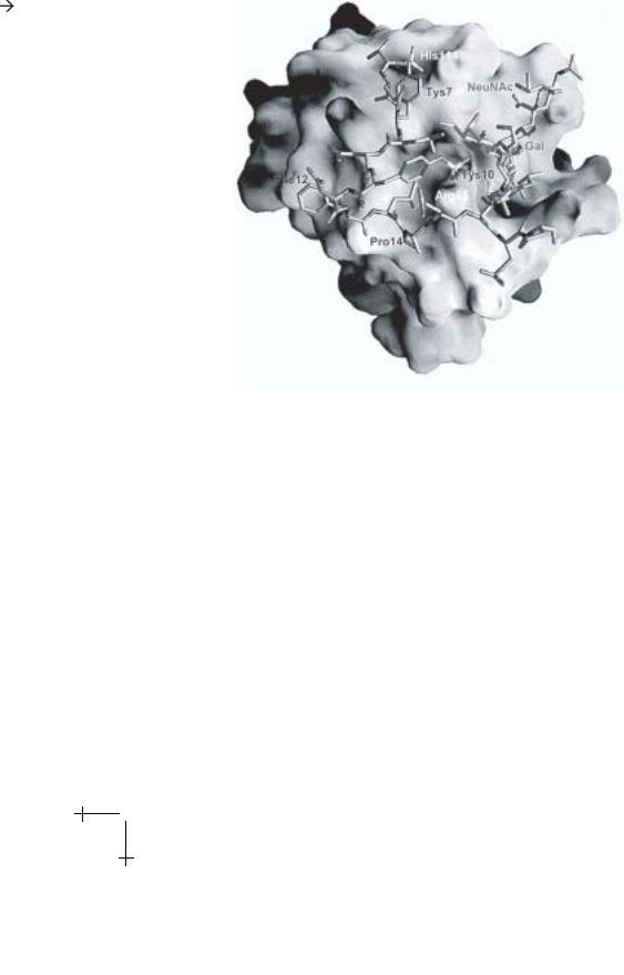
Fig. 1.1. Determined by X-ray di raction, a vertex (stick) representation shows the important 19 amino acid tip (SGP) of the mucin P-selectin glycoprotein ligand- 1 (PSGL-1) in its bound state conformation superposed on the van der Waals surface of the outer lectin domain of the cell membrane receptor P-selectin (taken from Somers et al. [29]).

or other small molecular residue. As an illustration, Figure 1.1 shows the structural complex obtained recently for the reactive tip of a glycosylated protein ligand bound to the outer protein domain of its cell surface receptor called P(for platelet)-selectin [29]. Essential in immune function, this interaction enables white blood cells to transiently stick and carry out a rolling patrol of the vascular wall under high shear stress in blood vessels. Referred to as a carbohydrate-protein bond, this ligand-receptor interaction is comprised of several sugar-peptide and sulfopeptide-peptide hydrogen bonds plus a metal-ion coordination bond spread over many residues of both the receptor lectin domain and the tip of the large glycoprotein ligand. Even so, association and dissociation of this ligand-receptor complex in solution

150	Physics of Bio-Molecules and Cells

seems to exhibit first order kinetics as expected for an ideal “bond”, which is modeled as a bound state confined by a single energy barrier. Furthermore, from force probe tests, we will also see that a single barrier dominates the kinetics of dissociation over many orders of magnitude in time scale for this complex interaction. Yet, probe tests of other species of the same class of bonds reveals that a sequence of barriers impede dissociation in di erent ranges of force. Thus, the landscape of energy barriers in a complex interaction can produce highly specialized dynamic responses in molecular reactions and linkages under stress, which is a principal design requirement for chemistry in living systems. An important step towards understanding these designs lies in probing the relation between force – time – chemistry at the level of single molecules.

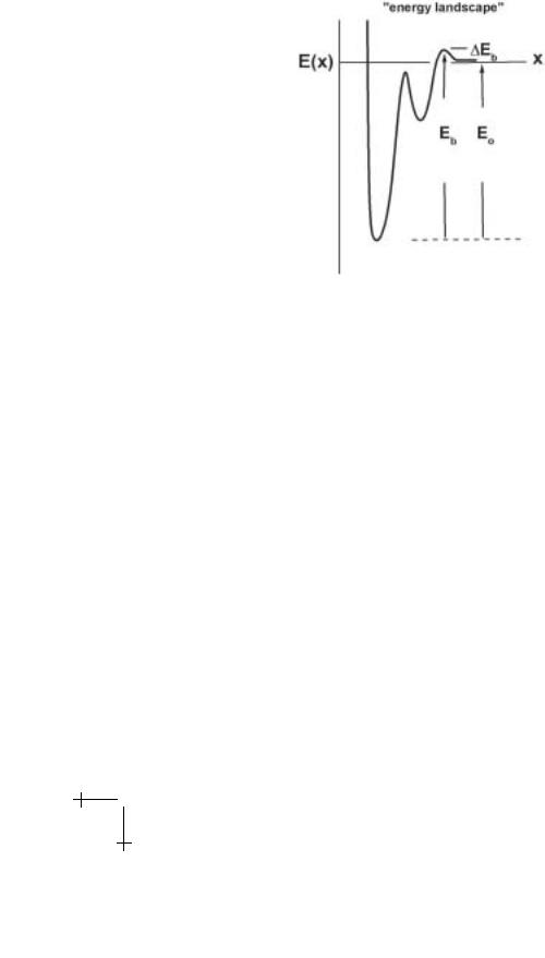
In this tutorial, our aim is to show that measuring forces to pull apart single biomolecular complexes over an enormous span of time scales provides a spectroscopic method to explore the energy landscape of barriers which govern dissociation kinetics. By landscape, we mean the free energy profile along a preferential pathway (or pathways) followed most often through configuration space during dissociation; other pathways involve significantly greater energy, which makes their traverse extremely rare. Thus, an energy landscape is viewed to start from a minimum representing the bound state and rise over one or more peaks with intervening valleys to reach the dissociated state as illustrated schematically in Figure 1.2. The peaks are local saddle points in the energy surface and define barriers to kinetics. Because of the thermal (Boltzmann) weighting of the energy barriers, the most prominent barrier is the dominant impedance to kinetics with little retardation to dissociation from passage of lower barriers. When a bond or molecular complex is pulled apart under a ramp of force in a probe test, the barriers diminish in time and thus unbonding force depends on rate of loading (= force/time). As a consequence of diminishing barrier heights, the most frequent forces for unbonding plotted on a scale of log(loading rate) yield a dynamic spectrum that images the hierarchy of energy barriers traversed along the force-driven pathway [7, 10]. Thus, the method of dynamic force spectroscopy (DFS) probes the inner world of molecular interactions.

1.1.3 Biochemical and mechanical perspectives of bond strength

Given the conceptual energy landscape shown in Figure 1.2, it is useful to compare traditional ways of characterizing the strength of chemical bonds. Starting with biochemistry, the scale for bond strength is usually taken as the free energy di erence E0 between bound and free states – or “binding” energy. In an ideal-dilute solution, the binding energy sets the equilibrium partition of “bound-to-free” constituents, i.e. the mole fraction of bound complexes vw [AB] divided by the product of free reactants vw [A] vw [B],

E. Evans and P. Williams : Dynamic Force Spectroscopy

151

Fig. 1.2. Conceptual energy profile along a scalar reaction coordinate. In this hypothetical example, the energy landscape exhibits a primary bound state and a secondary metastable state punctuated by two energy barriers. From the perspective of biochemistry, only the outer barrier Eb and binding energy E0 = Eb −∆Eb are important in bond formation and dissociation.

where concentrations [number/volume] are converted to a scale of mole fraction by the partial molar volume of water vw (e.g. one liter per 55 Moles). At equilibrium, the ratio Keq = [AB]/{vw[A][B]} expresses the thermodynamic balance, kBT log(Keq) = E0, between reduction in (mixing) entropy and gain in free energy from binding. The important dynamical corollary to thermodynamic equilibrium is “detailed balance” where the number of complexes that form per unit time Kon [A] [B] must exactly equal the number that dissociate per unit time Ko [AB]. The “on” rate Kon (M−1 time−1) and “o ” rate Ko (time−1) are empirically-defined parameters.

As such, the connection between equilibrium thermodynamics and phenomenological kinetics is through what’s called the dissociation constant KD = Ko /Kon, which has units of concentration and is inversely related to the equilibrium constant, i.e. 1/Keq = vw KD.

Consistent with the label, lowering the concentration of reactants below KD leads to complex dissociation and increasing concentration promotes complex formation. Introduced by Van’t Ho and Arrhenius in the late 19th century [16], the long-held phenomenological view is that kinetic rates start with primitive-attempt rates driven by molecular excitations but then are discounted dramatically by an inverse exponential (Arrhenius)

152	Physics of Bio-Molecules and Cells

dependence on a dominant energy barrier. For instance, once the reacting molecules come together rapidly by di usion, the entrance barrier ∆Eb shown in Figure 1.2 would retard association on approach to the bound state, i.e. Kon exp(−∆Eb/kBT ). Likewise, given that inner barriers are more than kBT lower, the height Eb of the paramount-outer barrier relative to the primary minimum would govern the rate of dissociation, i.e. Ko exp(−Eb/kBT ). Since the di erence Eb − ∆Eb in energy barriers equals the binding energy E0, the ratio of kinetic rates is consistent with “detailed balance” at equilibrium. However, what’s clearly missing in this biochemical perspective of bond strength is force!

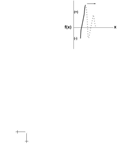
Fig. 1.3. Schematic of the force (solid curve) required to displace molecular components of a bond given the conceptual energy landscape in Figure 1.2. From the viewpoint of mechanics, the complex should become unstable and dissociate from the location of the steepest energy gradient just beyond the primary minimum. The remainder of the energy landscape (dotted curve) would appear not to a ect bond strength.

In contrast to the biochemical perspective, classical mechanics is precise in its prescription of bond force. Specifically, the force required to separate interacting molecules is the gradient in energy along the landscape (or interaction potential). The subtlety is that not all positions along the energy profile are accessible as we apply increasing force to pull molecules apart. As sketched in Figure 1.3, only regions of the energy contour with monotonically-increasing gradients would be stable under rising force, which could leave major portions of the landscape as “virtual” or unmapped by a pulling force. Once force exceeds the steepest gradient in energy (just beyond the primary minimum in Fig. 1.2), the molecules would jump apart. Hence, from a mechanical perspective, bond strength is independent of

E. Evans and P. Williams : Dynamic Force Spectroscopy

153

barrier heights or features of the landscape other than the maximum gradient. Here, what’s missing is time and temperature!

1.1.4 Relevant scales for length, force, energy, and time

At the beginning, it is important to introduce the relevant length, force, energy, and time scales appropriate to measurements of single bond properties. The increment of length is obviously the size of a small molecule, which is taken as a nanometer (about three water molecules end-to-end). One nanometer is comparable to the mean spacing between molecules at a concentration of 1 mole/liter and five hundred-fold smaller than the wavelength of green light. Next, the characteristic scale of force needed to speed up dissociation and quickly break weak-noncovalent bonds is a piconewton (pN). One piconewton is about one ten-billionth of a gram weight (10−10 gm) or ten thousand-fold smaller than can be measured with an analytical microbalance. The product of length and force scales reveals the appropriate scale for energy – thermal energy kBT – which is 4 pN nm at biological temperatures ( 300 K), which is better known as 0.6 Kcal/mole for Avogadro’s number ( 6 × 1023) of molecules.

Time scale is a much more complicated issue. At the atomic level, the time scale for excitations is typically 10−15 s or comparable to the frequency of the light photons emitted or adsorbed in atomic transitions. Much longer, however, kinetics in vacuum or gas phase reactions are theorized to start at an attempt frequency defined by thermal energy over Planck’s constant, kBT /h 1013/s. This frequency characterizes thermally-driven transitions in a quantum oscillator model of chemical dissociation as developed by Eyring [16]. However, in condensed liquids or inside compact structures like proteins, kinetics are slowed significantly by dissipative collisions between and within the molecular components as well as with the myriad of other molecules in the surrounding solvent. For example, an instantaneous impulse of momentum from a thermal collision in water will die out on a time scale of 10−12 s or less as set by the ratio of damping to molecular inertia. Because of damping, many impulses are needed to separate molecular components over a distance comparable to the scale of bond length even in the absence of a bonding interaction.

Hence, as will be shown next, kinetics in the overdamped world of biomolecular interactions begin on a time scale set by a di usive relaxation time for the bond. This relaxation time is on the order of 10−9 s which means that attempt frequencies for unbonding in liquids are four orders of magnitude slower than predicted by vacuum theory. The corresponding attempt frequency of 109/s is then diminished many orders of magnitude by bond chemistry to reach laboratory kinetic rates of as long as 1/month or more for dissociation of weak biomolecular interactions – i.e. a range

154	Physics of Bio-Molecules and Cells

of more than sixteen orders of magnitude in time scale! Most important, this enormous span in time scale corresponds to breakage forces that range from the maximum gradient in the molecular interaction potential ( nN) under nanosecond detachment to zero force under detachment slower than the spontaneous dissociation rate 1/to .

1.2 Brownian kinetics in condensed liquids: Old-time physics

To make the connection between force – time – and chemistry, we need to review the physics that underlies kinetics in a liquid environment. Motivated by Einstein’s theory of Brownian motion [6], these well-known developments take advantage of the huge gap in time scale that separates rapid thermal impulses in liquids (<10−12 s) from slow processes in laboratory measurements. Three equivalent formulations describe molecular kinetics in an overdamped environment (see for example, N.G. van Kampen: Stochastic Processes in Physics and Chemistry [33]). The first is a nanoscopic description where molecules behave as particles with instantaneous positions or states x(t) governed by an overdamped Langevin equation of motion,

dx/dt = [f + δf ]/ζ.

(1.1)

Changes in state are driven by instantaneous force scaled by the mobility of states or inverse of the damping coe cent ζ. The deterministic part of the force (f = − E + fext) includes the local gradient in molecular interaction potential E(x) plus the applied external force fext. To this is added a random-uncorrelated force δf that embodies the many body collisions associated with the thermal environment. These random impulses are governed by the ßuctuation-dissipation theorem, δf2 ∆t kBT ζ. (Einstein’s great insight was to recognize that the average mechanical energy imparted by thermal impulses had to equal thermal energy, i.e. the ensemble-average integral of mechanical power ∆t δf · δv dt = kBT . The assumption of overdamped motions δv = δf/ζ then yields the autocorrelation relation that governs force fluctuations.) The nanoscopic view can also be described by a stochastic process, which has become the foundation for an important computational technique – Brownian dynamics or dissipative Monte-Carlo simulations (referred to by its creators as “smart Monte-Carlo” [27]). In this description, the likelihood P (x+∆x, t+∆t|x, t) that a state x(t) will evolve to a new state x + ∆x over a time increment ∆t is the product of the equilibrium (long-time) Boltzmann weight for the step and a di usive-Gaussian weight for dynamics,

P (t → t + ∆t) exp{−[∆E − fext · ∆x]/kBT }

× exp{−|∆x − f∆t/ζ|2/(4D∆t)}/(D∆t)1/2 (1.2)

E. Evans and P. Williams : Dynamic Force Spectroscopy

155

where the di usivity of states D is taken here to be a constant given by the Einstein–Stokes relation, D = kBT /ζ. Finally, on time scales that include many thermal impulses ( 10−9 s and longer), the overdamped dynamics can be cast in a continuum theory where the density of states ρ(x, t) at location x and time t evolves according to the Smoluchowski transport equation,

dρ/dt = − · J

(1.3)

with the ßux of states J = (fext − E)ρ/ζ −D ρ defined by force-driven convection plus the di usive gradient. Although each description illuminates

di erent features of kinetics in a dissipative environment, Kramers [16, 18] demonstrated that Smoluchowski transport can be used to predict the rate for thermally-activated escape from a deeply bound state.

1.2.1 Two-state transitions in a liquid

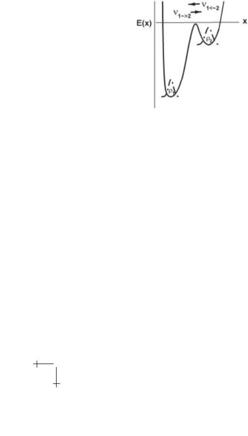
To illustrate the important features of chemical kinetics in liquids and the utility of Kramers approach, we begin by examining two-state transitions with an energy landscape modelled by two deep energy minima separated by an intervening barrier (Fig. 1.4). In this 1-D abstraction, a scalar coordinate “x” is assumed to map the transition pathway over a barrier at energy Ets relative to the deepest minimum. Following Kramers, rates of transition between these two states are approximated by stationary fluxes (constant #/time) between the states under appropriate boundary conditions,

J = −D[(∂E/∂x)ρ/kBT + ∂ρ/∂x] = constant.

(1.4)

Again treating the di usivity or mobility of states as locally constant, integration of the stationary flux relates flux to the end-state densities (ρ1, ρ2),

J = D{ρ1 exp(E1/kBT ) − ρ2 exp(E2/kBT )}/ dx exp[E(x)/kBT ] ·

1→2

(1.5)

Directional rates of transition ν1→2 and ν1←2 between the two states are then found by starting with all states essentially at “1” or “2” and an adsorbing boundary at the final state “2” or “1” (i.e. ρ2 = 0 or ρ1 = 0). This leads to the expressions for forward and reverse rates of transition,

ν1→2	= Dρ1 exp[(E1	− Ets)/kBT ]/Lts
ν1←2	= Dρ2 exp[(E2	− Ets)/kBT ]/Lts.	(1.6)

Energy-weighted, the major contribution to the pathway integral in equation (1.5) arises local to the transition state and defines a length scale

156	Physics of Bio-Molecules and Cells

Fig. 1.4. Conceptual energy landscape for a two-state transition.

for barrier width, Lts ≡ 1↔2 dx exp[(E(x) − Ets)/kBT ]. As expected, “detailed balance” (ν1→2 = ν1←2) yields the ratio (ρ1/ρ2)∞ = exp[(E2 −

E1)/kBT ] required for densities of states at long times.

1.2.2 Kinetics of first-order reactions in solution

Another revealing application of Kramers theory is to bimolecular reactions (A + B ↔ AB) in solution. Here, we imagine that a 1-D density ρA (#/length) of reactant (e.g. A) exchanges with the bound state (reactant B) at one end of a scalar coordinate x as sketched in Figure 1.5. As such, the reverse rate in equation (1.6) predicts the rate of capture by the attractive potential:

νB←A ≈ DρA exp[−∆Eb/kBT ]/Lts

(1.7)

which may involve passage of an entrance barrier ∆Eb like that sketched in Figure 1.5. To connect with the solution in 3-D beyond the reaction pathway, the 1-D density ρA is modelled as the product of solution concentration cA (number/volume) and the e ective cross section of the reactive site, i.e. ρA 4πx2bcA. In this way, the bimolecular “on” rate in solution is found from the rate of capture per concentration of reactant A, i.e. Kon = νB←A/cA. Since barrier width Lts will be comparable to barrier location xb, “on” rate in solution can be approximated by,

Kon (4π “xbD”) exp[−∆Eb/kBT ].

(1.8)

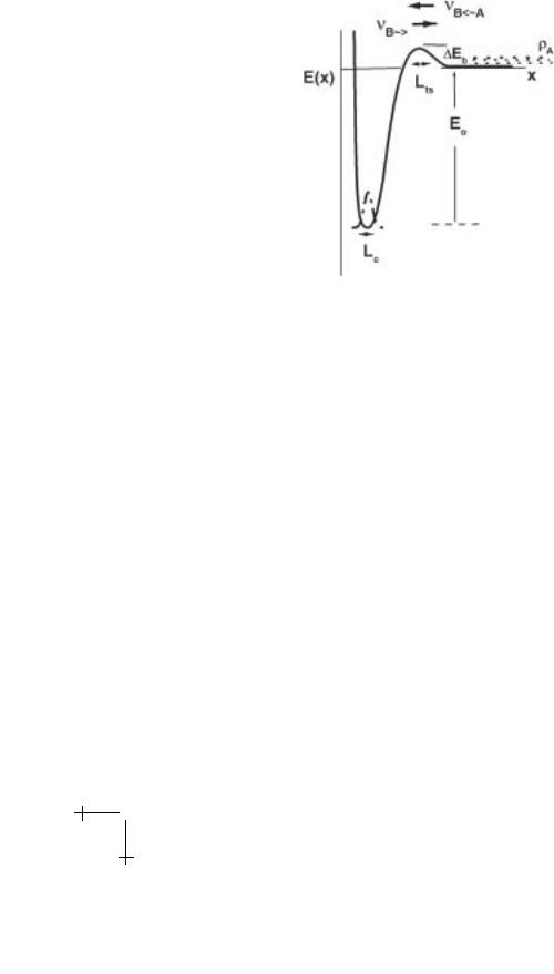
E. Evans and P. Williams : Dynamic Force Spectroscopy

157

Fig. 1.5. Conceptual energy landscape for capture and release of components in solution.

The prefactor 4π“xbD” in equation (1.8) represents the well-known Smoluchowski rate for di usion-controlled aggregation which, for twospheres (A–B), is given by the product of interparticle separation (“xb” = rA + rB) at contact and combined particle di usivity, (“D” = DA + DB). For nanometer-size molecules in water, the Smoluchowski scale for “on” rate is 109−1010 M−1 s−1, whereas typical “on” rates for macromolecular interactions are only 106 M−1 s−1. Thus, formation of macromolecular bonds appears to involve entrance barriers of 10kBT in energy.

In examining the “o ” rate, the crucial concept is that the constituents in a bound complex are driven to escape by entropy confinement. In 1- D, the relevant entropy gradient is determined by the density of states ρ1 (#/length) local to the minimum. Under strong confinement, the distribution of states ρ(x) = ρ1 exp[−(E − E0)/kBT ] diminishes rapidly away from

the minimum and, hence, the integral	1 ρ(x)dx ≈ 1 relates the entropy
			1			−		−
gradient to a confinement length, i.e. ρ1 = 1/Lc and Lc =				exp[			(E
E		(1.6)			yields a
0)/kBT ]dx. Introducing this length	scale into equation
generic expression for “o ” rate (1/to = νB→∞),
νB→∞ = D exp(−Eb/kBT )/LcLts							(1.9)

where kinetics are driven by a di usive attempt frequency D/LcLts and attenuated by the classic Arrhenius dependence on barrier energy Eb. Because of near-thermodynamic equilibration on a local scale, confinement