Micro-Cap v7.1.6 / Ug

		Expand: This command expands the text field where the text cursor is into a
		large dialog box for editing or viewing. To use the feature, click the mouse in
		the desired text field, and then click the Expand button.
		Stepping: This command invokes the Stepping dialog box. Stepping is
		covered in a separate chapter.
		Properties: This command invokes the Properties dialog box which lets you
		control the analysis plot window and the way curves are displayed.
		Help: This command invokes the Help Screen. The Help system provides
		information by index and topic.
		The Numeric limits field provides control over the analysis time range, time step,
	Numeric limits
		number of printed points, and the temperature(s) to be used.
		• Time Range: This field determines the start and stop time for the analysis.
		The format of the field is:
		<tmax> [,<tmin>]
		The run starts with time set equal to <tmin>, which defaults to zero, and ends
		when time equals <tmax>.
		• Maximum Time Step: This field defines the maximum time step that the
		program is allowed to use. The default value, (<tmax>-<tmin>)/50, is used
		when the entry is blank or 0.
		• Number of Points: The contents of this field determine the number of
		printed values in the numeric output. The default value is 51. Note that this
		number is usually set to an odd value to produce an even print interval. The
		print interval is the time separation between successive printouts. The print
		interval used is:
		print interval = (<tmax> - <tmin>)/([number of points] - 1)
		• Temperature: This field specifies the global temperature of the run. This
		temperature is used for each device unless individual device temperatures are
		specified. If the Temperature list box shows Linear the format is:
		<high> [ , <low> [ , <step> ] ]

85

Curve options

Expressions

Variables list

The values are in degrees Celsius. The default value of <low> is <high>, and the default value of <step> is <high> - <low>.

If the Temperature list box shows List the format is:

<t1> [ , <t2> [ , <t3> ] [ ,...]]

where t1, t2,.. are individual values of temperature.

One run is produced for each requested temperature, producing multiple branches of each curve.

The Curve options field is located below the Numeric limits field and to the left of the Expressions field. Each curve option affects only the curve in its row. The options function as follows:

The first option toggles the X-axis between a linear and a log plot. Log plots require positive scale ranges.

The second option toggles the Y-axis between a linear and a log plot. Log plots require positive scale ranges.

The option activates the color menu. There are 64 color choices for an individual curve. The button color is the curve color.

The option prints a table of the curve's numeric values. The number of values printed is set by the Number of Points value. The table is printed to the Numeric Output window and saved in the file CIRCUITNAME.TNO.

A number from 1 to 9 in the (P) column places the curve into a numbered plot group. All curves with like numbers are placed in the same plot group. If the P column is blank, the curve is not plotted.

The X Expression and Y Expression fields specify the horizontal (X) and vertical

(Y) expressions. MC7 can evaluate and plot a wide variety of expressions for either scale. Usually these are single variables like T (time), V(10) (voltage at node 10), or D(OUT) (digital state of node OUT), but the expressions can be more elaborate like V(2,3)*I(V1)*sin(2*PI*1E6*T).

Clicking the right mouse button in the Y expression field invokes the Variables list which lets you select variables, constants, functions, and operators, or expand

86 Chapter 4: Transient Analysis

the field to allow editing long expressions. Clicking the right mouse button in the other fields invokes a simpler menu showing suitable choices.

The X Range and Y Range fields specify the numeric scales to be used when plotting the X and Y expressions.

The format is:

<high> [,<low>] [,<grid spacing>] [,<bold grid spacing>]

<low> defaults to zero. [,<grid spacing>] sets the spacing between grids. [,<bold grid spacing>] sets the spacing between bold grids. Placing "AUTO" in the scale range calculates that individual range automatically. The Auto Scale Ranges option calculates scales for all ranges during the simulation run and updates the X and Y Range fields. The Auto Scale (F6) command immediately scales all curves, without changing the range values, letting you restore them with CTRL + HOME if desired. Note that <grid spacing> and <bold grid spacing> are used only on linear scales. Logarithmic scales use a natural grid spacing of 1/ 10 the major grid values and bold is not used. The Auto Scale command uses the Preferences / Auto Scale Grids value to set the grid spacing if none is specified in the range.

These options include the following:

Transient options

•Run Options

•Normal: This runs the simulation without saving it.

•Save: This runs the simulation and saves it to disk, using the same format as in Probe. The file name is CIRCUITNAME.TSA.

•Retrieve: This loads a previously saved simulation and plots and prints it as if it were a new run. The file name is CIRCUITNAME.TSA.

•State Variables

These options determine the state variables at the start of the next run.

• Zero: This sets the state variable initial values (node voltages, inductor currents, digital states) to zero or X.

87

•Read: This reads a previously saved set of state variables and uses them as the initial values for the run.

•Leave: This leaves the current values of state variables alone. They retain their last values. If this is the first run, they are zero. If you have just run an analysis without returning to the Schematic editor, they are the values at the end of the run. If the run was an operating point only run, the values are the DC operating point.

•Operating Point: This calculates a DC operating point. It uses the initial state variables as a starting point and calculates a new set that represents the DC steady state response of the circuit to the T=0 values of all sources.

•Operating Point Only: This calculates a DC operating point only. No transient run is made. The state variables are left with their final operating point values.

•Auto Scale Ranges: This sets the X and Y range to AUTO for each new analysis run. If it is not enabled, the existing scale values from the X and Y Range fields are used.

The Run, State Variables, and Analysis options affect the simulation results. To see the effect of changes of these options you must do a run by clicking on the Run command button or pressing F2.

88 Chapter 4: Transient Analysis

Note: MC7 initiallyselects the voltage curves of the first two named nodes for plotting.

Selecting curves to plot or print

MC7 automatically creates a set of analysis limits for newly created circuits. It tries to guess what curves you may want to look at and what plot and analysis options you may want. Usually, it is necessary to change these initial guesses.

Changes you make to any entry in the Analysis Limits dialog box are saved with the circuit file, so you don't need to enter these each time you run.

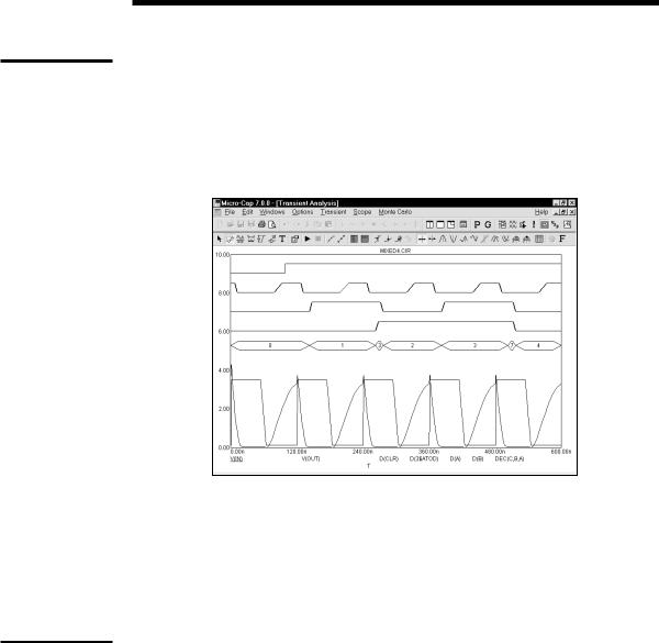
Click on the Run button to do the transient analysis of the MIXED4 circuit.

Plotting other curves

Figure 4-2 Transient analysis of MIXED4

The top five curves are digital and show the CLR input, clock input, the state outputs of the first two flip-flops, and the decimal value of the three flip-flop outputs. The next two curves are plots of the voltage at the input pulse source and the output of the analog section. In general, V(A) plots the voltage on an analog node A. D(B) plots the state of a digital node B.

You can plot expressions using a variety of variables such as node voltage or device terminal voltage or current. To plot different curves, you can add new curve fields or you can change existing ones. To illustrate, press F9 to display the Analysis Limits dialog box. Click in any column of the last row. Click the Add button in the upper part of the dialog box. This adds a new curve row and moves the text cursor to the P column of the new row. It also duplicates the contents of all fields of the row above. Click the Delete button. This deletes the curve just added. Click the Add button to add the curve row back. Since we want the new

89

curves to be placed on a separate plot group, change the '1' in the P column to '2'. Press the Tab key twice or click the mouse in the Y Expression field. Type in the following:

"IC(Q4)*VCE(Q4)"

Use the Variables list to select hard-to- remember function and variable names.

Press the Tab key twice to move the cursor to the Y Range field and type "Auto". This tells the program to determine the Y scale range automatically, after the run. During the run, MC7 uses a default scale to start the plot. Several times during the run it will revise the scales based upon the curves. When the run is complete, MC7 determines the scale necessary to show the complete curves, plots it, and enters the new scales into the X and Y range fields.

If you can't remember the variable or function name you want, use the Variables list as a memory aid. To illustrate, click the Add button again. Click in the new Y Expression field with the left mouse button and drag select the entire Y expression. Click on this selected Y expression with the right mouse button. This invokes the Variables list, a small pop-up menu that lets you select variables, functions, and operators. It also lets you expand the limited text editing area to a full size text edit dialog box. This is handy for complex expressions with many parentheses. Click on Variables and then on Device Currents. This displays a dialog box with a list of the available device currents in the circuit. Click on I(VCC), then on OK. The text "I(VCC)" is entered in the Y Expression field and the cursor is placed to the right of the text. The Y expression will now look like this:

I(VCC)

Type "*". Click the right mouse button and select Variables / Device Voltages / V(VCC). Click OK. The Y expression should now look like this:

I(VCC)*V(VCC)

Press the Home key to move the cursor to the start of the field. Click the right mouse button and click Functions / Calculus / SUM. SUM is the integration operator. It integrates the expression to the right of the text cursor, with respect to the X expression variable, T. Press the End key to put the cursor at the end of the field and type "/T". This produces an expression for the average power supplied by the VCC battery. The Y expression should now look like this:

SUM(I(VCC)*V(VCC),T)/T

Since the new curve was created with AUTO in the Y Range field we do not

90 Chapter 4: Transient Analysis

need to edit that field. After the run, MC7 will determine the actual range and calculate a suitable Y scale. Because there are two curves sharing the same plot group, it can do this two ways; 1) by finding a common scale large enough to show all of both graphs, or 2) by finding an individual scale for each curve and printing two Y scales. The choice is determined by the Same Y Scales option on the Scope menu. If this option is checked, then all curves in each plot group will share a common scale large enough to plot all parts of each curve. This is true regardless of whether auto or user-specified scales are used. If you select this option, MC7 draws a single scale using the largest of the specified or calculated scales. Click the Run button. Here is how the new run looks when the option is disabled.

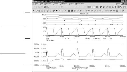
Plot group 1

Plot group 2

Figure 4-3 Transient analysis with two plot groups

Group 1 contains the original curves. Group 2 contains the new curves: the instantaneous collector power of the output transistor Q4, and the average power supplied by the VCC battery. Plot grouping is specified by the P column number. All curves with the same number are plotted in the same group.

Analog and digital curves may be grouped together or separately. When grouped together, digital curves are plotted in the same order they occur in the dialog box, starting at the top of the graph. Analog curves are plotted using the range scales, which only apply to analog curves. This can cause the curves to overlap. Overlap can be minimized by compressing the analog curves with a large Y Range value. Separating analog and digital curves into groups avoids overlap but is less convenient when comparing the two sets of curves at the same time value.

91

Same Y Scales

Tokens Option

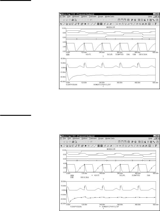
To see what the curves would look like with common Y scales, enable the Same Y Scales option on the Scope menu. This is what the plots look like:

Figure 4-4 The plot with the Same Y Scales option enabled

The two scales have been collapsed into a common scale, containing the largest and smallest scale value from each.

While color identifies individual curves, black and white printers create plots where it is hard to tell the curves apart. Tokens can help identify the different

curves. To illustrate, click on the Tokens button .

Figure 4-5 The plot with tokens

92 Chapter 4: Transient Analysis

The Plot Properties dialog box

Curve display and format can be changed with the Plot Properties dialog box. Press F10 to invoke the dialog box for the plot. It looks like this:

Figure 4-6 The Properties dialog box

Click on the V(OUT) curve and the Colors, Fonts, and Lines tab. From the Curve Line group select a width of 3. For the V(IN) plot select the third pattern in

the list. Click the OK button. Disable tokens by clicking the Tokens button in the Tool bar. The screen should look like this:

Figure 4-7 Using line width and pattern

93

The Plot Properties dialog box lets you control the analysis plot window. It is especially useful for controlling how curves are displayed after or even before the plot. Before a plot exists, you can access this dialog box by clicking on the Properties button (Press Esc to remove the Analysis Limits dialog box if present). The dialog box provides the following choices:

•Plot

•Curves: This list box lets you select the curve that the Plot and Graph fields apply to.

•Title: This field lets you specify what the plot title is to be.

•Curve: This group's check box controls whether the curve will be plotted or not. If you want to delete the curve from the plot group, remove the check mark by clicking in the box.

•Plot Group: This list box controls the plot group number.

•Plot Type: This list box controls the plot type. The three available types include rectangular, Smith Chart, and polar. Only rectangular is available for transient analysis.

•Scales and Formats

•Curves: This lets you select the curve that the other fields apply to.

•X: This group includes:

•Range Low: This is the low value of the X range used to plot the selected curve.

•Range High: This is the high value of the X range used to plot the selected curve.

•Grid Spacing: This is the distance between X grids.

•Bold Grid Spacing: This is the distance between bold X grids.

•Scale Format: This accesses a dialog box where you select the numeric format used to print the X axis scale.

94 Chapter 4: Transient Analysis