Micro-Cap v7.1.6 / Ug

Numeric output

To obtain a tabulation of the numerical values simply click the Numeric Output button for each curve for which numeric output is desired. Do that now for

the first two curves. Press F9, then click the buttons. Press F2 to run the analysis. All text or numeric output is directed to the Numeric Output window and to a disk file with the name DIFFAMP.ANO. Press F5 to see the window. The first part shows the results of the DC operating point. Scroll down to see the numeric values for the curves. The display should look like this:

Figure 5-7 Numeric output

A printout of the data in the Numeric Output window may be obtained from the Print option of the File menu.

To display the Analysis Plot window, press F4, or click on the Analysis Plot button .

To display the Output window, press F5, or click on the Numeric Output button

.

Disable the numeric output button for each curve.

115

Noise plots

MC7 models three types of noise; thermal, shot, and flicker noise.

Thermal noise is produced by the random thermal motion of electrons and is always associated with resistance. Discrete resistors and the parasitic resistance of active devices contribute thermal noise.

Shot noise is caused by a random variation in the production of current from a variety of sources including recombination and injection. It is usually associated with dependent current sources. All semiconductor devices generate shot noise.

Flicker noise comes from a variety of sources. In BJTs, the source is contamination traps and other crystal defects that randomly release their captured carriers.

Noise analysis computes the contribution from all these sources as seen at the input and output. Output noise is calculated at the output node specified in the Noise Output field. To plot it, specify ONOISE as the Y expression. Input noise is calculated at the same output node(s) specified in the Noise Output field, but is divided by the gain from the node(s) specified in the Noise Input field to the output node. To plot or print input noise, specify INOISE as the Y expression.

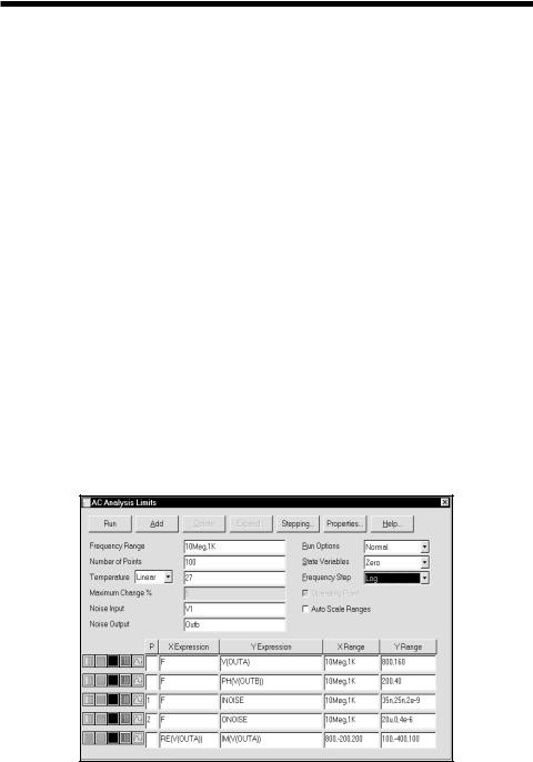
Press F9 and edit the analysis limits to match Figure 5-8. Be sure to disable numeric output for the first two curves and to select the Log option.

Figure 5-8 The Analysis Limits for Noise plots

116 Chapter 5: AC Analysis

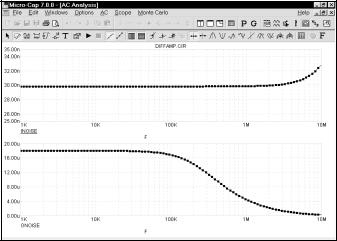
Press F2 to run the analysis. The results look like this:

Figure 5-9 Plots of input and output noise

In this circuit, thermal noise is generated by the resistors. Shot and flicker noise are generated by the transistors.

Because the equations are structured differently for noise, it is not possible to simultaneously plot noise variables and other types of variables such as voltage and current. That is why we disabled the other curves by placing a blank in their P fields. If you attempt to plot both noise and other variables, the program will issue an error message.

Noise is an essentially random process and as a result carries no phase information. For this reason, noise is defined as an RMS quantity. Thus the phase (PH) and group delay (GD) operators will not produce meaningful results when plotting noise. With noise, only magnitudes are meaningful.

The units of noise are V / sqrt(Hz).

117

Nyquist plots

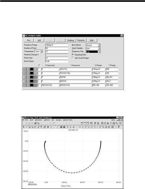
A Nyquist plot is easy to generate. Edit the analysis limits to look like these. Here we have enabled the last curve and disabled the other curves and selected log stepping.

Figure 5-10 Analysis limits for the Nyquist plot

Press F2 to run the analysis. The result looks like this:

Figure 5-11 The Nyquist plot

Note that the X expression in this case was RE(V(OUTA)), not F as it usually is. In general, it can be any expression involving any AC variable.

118 Chapter 5: AC Analysis

Smith charts

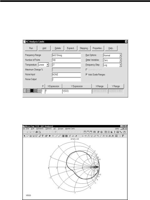
To generate a Smith chart plot, select the option adjacent to the P column. Here is what the Analysis Limits dialog box looks when set up to create a Smith chartplot.

Figure 5-12 Analysis limits for the Smith chart

Here is what a typical Smith chart plot looks like:

Figure 5-13 Typical Smith chart plot

119

Polar plots

To generate a polar plot, select the option adjacent to the P column. Here is what a typical polar plot Analysis Limits dialog box looks like:

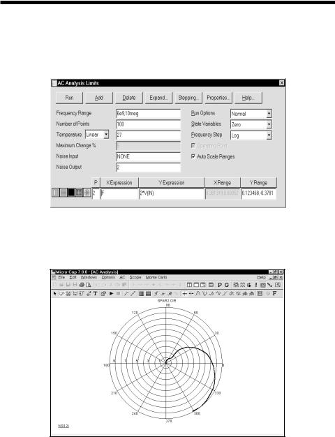
Figure 5-14 Analysis limits for a polar plot

Here is what a typical polar plot looks like:

Figure 5-15 Typical polar plot

120 Chapter 5: AC Analysis

Chapter 6

DC analysis

What's in this chapter

DC analysis is the topic for this chapter. It is a short tutorial covering these subjects:

•What DC analysis does

•What the DC analysis limits do

•A simple circuit for generating IV-curves

121

DC analysis

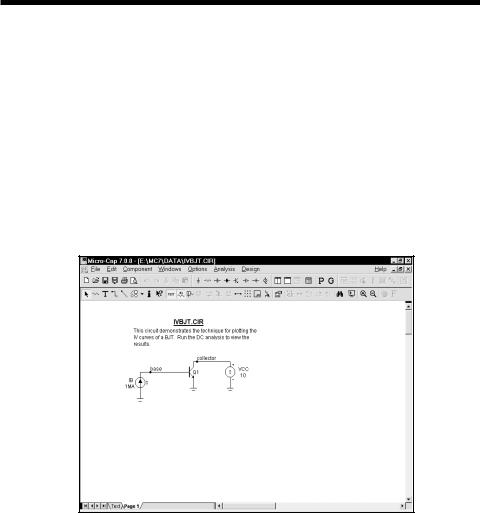
In DC analysis, the program treats capacitors as open circuits and inductors as short circuits. It sweeps the specified Variable 1 and solves for the steady-state DC node voltages and branch currents. Two stepping loops are provided for easy creation of parametric plots such as device IV curves. The variable for either loop can be a voltage or current source value, temperature, a model parameter, or a symbolic variable. As in the other analysis routines, the complete set of variables are available for printing and plotting, with the obvious exceptions of charge, flux, capacitance, inductance, B field, and H field. These variables are not provided since flux and charge are ignored in DC analysis. To explore DC analysis, load the file IVBJT. It looks like this:

Figure 6-1 The IVBJT circuit

This circuit is used to plot the I-V characteristics of a bipolar transistor. It can be easily adapted to other device types, such as GaAsFets, MOSFETs, and JFETs. There is a voltage source for the collector voltage sweep and a current source for the base current sweep.

After loading the circuit, select DC from the Analysis menu. When the DC Analysis Limits dialog box comes up, it looks like Figure 6-2.

122 Chapter 6: DC Analysis

Command buttons

Sweep group

Options

Curve options

Expressions

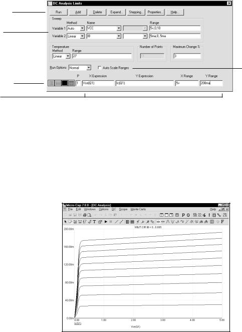
Figure 6-2 The DC Analysis Limits dialog box

The dialog box instructs MC7 to step the value of the current source IB from 0 to 5 ma, using a maximum step size of 0.5 ma. For each value of the current source, IB, the voltage source, VCC, is to be swept from 0 to 5 volts, using a maximum step size of 10. The step size may be varied during the run to optimize convergence and to conform to the <Maximum change %> constraint, but it is never to be larger than 10. Click on the Run command button and the results look like this:

Figure 6-3 DC analysis plot of IV characteristics

123

The DC Analysis Limits dialog box

Command buttons

Sweep group

The Analysis Limits dialog box is divided into five major areas: the Command buttons, Sweep group, Curve options, Expression fields, and Options.

Command buttons provide these commands.

Run: This command starts the analysis run. Clicking the Tool bar Run button or pressing F2 will also start the run.

Add: This command adds another Curve options field and Expressions field line after the line containing the cursor. The scroll bar to the right of the Expressions field scrolls through the curves when needed.

Delete: This command deletes the Curve option field and Expressions field line where the text cursor is.

Expand: This command expands the working area for the text field where the text cursor currently is. A dialog box is provided for editing or viewing. To use the feature, click in an expression field, then click the Expand button.

Stepping: This command calls up the Stepping dialog box. Stepping is reviewed in a separate chapter.

Properties: This command invokes the Properties dialog box which lets you control the analysis plot window and the way curves are displayed. See

the Plot Properties dialog box article in Chapter 4, "Transient Analysis".

Help: This command calls up Help information for DC analysis.

The definition of each field in this group is as follows:

• Variable 1: This row specifies the Method, Name, and Range fields for Variable 1. Its value is usually plotted along the X axis. The column fields for this variable are:

• Method: This field specifies one of four methods for sweeping or stepping the variable: Auto, Linear, Log, or List.

• Auto: In this mode the rate of step size is adjusted to keep the point-to-point change less than Maximum Change % value.

124 Chapter 6: DC Analysis