

Micro-Cap v7.1.6 / Ug
.pdfDEV tolerances force the use of private libraries, regardless of the state of the PRIVATEANALOG or PRIVATEDIGITAL flags.
This sample specifies a 10% absolute and 1% relative BF tolerance:
.MODEL N1 NPN (BF=300 LOT=10% DEV=1%)
In this example, assuming a worst case distribution, the first N1 model is randomly assigned one of the two values 270 or 330. These two values are calculated from the mean value of 300 and 10% LOT tolerance as follows:
BF = 270 = 300 - .1•(300)
BF = 330 = 300 +.1•(300)
Suppose that the LOT toleranced BF value was randomly chosen to be 330. Then all N1 transistors, including the first, are randomly given one of these values, based upon the 1% DEV tolerance:
327 = 330 - .01•300
333 = 330 + .01•300
If the LOT toleranced BF value had been randomly chosen to be 270, then all N1 transistors, including the first, would be randomly given one of these values, based upon the 1% DEV tolerance:
267 = 270 - .01•300
273 = 270 + .01•300
Assuming a worst case distribution, all BF values in any particular run would be chosen from the set {267, 273} or the set {327, 333}.
Resistors, capacitors, and inductors can only be toleranced through their multiplier model parameter. The example below provides a 5% LOT tolerance and a .2% DEV tolerance for a capacitor.
.MODEL CMOD CAP(C=1 LOT=5% DEV=.2%)
Any capacitor that uses the CMOD model will be toleranced, since the toleranced C multiplier will multiply its capacitance value.
See the "Monte Carlo Analysis" chapter in the Reference manual for further information on using tolerances.
185

Distributions
The actual values assigned to a toleranced parameter depend not only on the tolerance, but on the distribution as well.
A worst case distribution places all values at the extremes of the tolerance band. There are only two values:
Min = Mean - Tolerance
Max = Mean + Tolerance
The mean value is the model parameter value.
A uniform distribution places values equally over the tolerance band. Values are generated with equal probability over the range:
From Mean - Tolerance to Mean + Tolerance
A Gaussian distribution produces a smooth variation of parameters around the mean value. Values closer to the mean are more likely than values further away. The standard deviation is obtained from the tolerance by this formula:
Standard Deviation = Sigma = (Tolerance/100)•Mean/SD
SD (from the Global Settings dialog box) is the number of standard deviations in the tolerance band. Thus, the standard deviation is calculated directly from the tolerance value. The value chosen depends upon how much of a normal population is to be included in the tolerance band. Here are some typical values:
Standard deviations |
Percent of population |
1.00 |
68.0 |
1.96 |
95.0 |
2.00 |
95.5 |
2.58 |
99.0 |
3.00 |
99.7 |
3.29 |
99.9 |
If you're certain that 99.9% of all 10% resistors are within the 10% tolerance, you would use the value 3.29. Using a Gaussian distribution, a 1K 10% resistor may have a value below 900 ohms or above 1100 ohms. The probability would be less than 0.1% for an SD of 3.29, but it could happen.
186 Chapter 10: Using Monte Carlo

Performance functions
MC7 saves all X and Y expression values of each plotted or printed expression at each data point for each run, so you can create histograms after the runs are done by picking a performance function and an expression. The performance function calculates a single number from the selected expression for each analysis run. All the numbers are combined to form a population which is statistically analyzed and its histogram is displayed. The performance functions supplied with MC7 include:
Rise_Time
Fall_Time
Peak_X
Peak_Y
Valley_X
Valley_Y
Peak_Valley
Period
Frequency
Width
High_X
High_Y
Low_X
Low_Y
X_Level
Y_Level
X_Delta
Y_Delta
X_Range
Y_Range
Slope
Phase_Margin
For a more detailed description of how the performance functions work see Chapter 7 of this book.
187

Options
The Monte Carlo options dialog box provides these choices:
•Status: Monte Carlo analysis is enabled by selecting the On button. To disable it, click the Off button.
•Number of Runs: The number of runs determines the confidence in the statistics produced. More runs produce a higher confidence that the mean and standard deviation accurately reflect the true distribution. Generally, from 30 to 300 runs are needed for a high confidence. The maximum is 30000 runs.
•Report When: This field specifies when to report a failure. The routine generates a failure report in the numeric output file when the Boolean expression in this field is true. The field typically contains a performance function specification. For example, this expression
Rise_Time(V(1),1,1,0.8,1.4)>10ns
would generate a report when the specified rise time of V(1) exceeded 10ns. The report lists the model statement values that produced the failure. These reports, included in the numeric output file (CIRCUITNAME.TNO for transient, CIRCUITNAME.ANO for AC, and CIRCUITNAME.DNO for DC), can be viewed directly and are also used by the Load MC File item in the File menu to recreate the circuits that created the performance failure.
• Distribution to Use: This choice controls the type of distribution used to generate the individual populations of component parameters.
• Gaussian distributions are governed by the standard equation
f(x) = e-.5•s•s/σ (2 •π ).5
Where s = x-µ /σ and µ is the nominal parameter value, σ is the standard deviation, and x is the independent variable.
•Uniform distributions have equal probability within the tolerance limits. Each value from minimum to maximum is equally likely.
•Worst case distributions have a 50% probability of producing the minimum and a 50% probability of producing the maximum.
188 Chapter 10: Using Monte Carlo
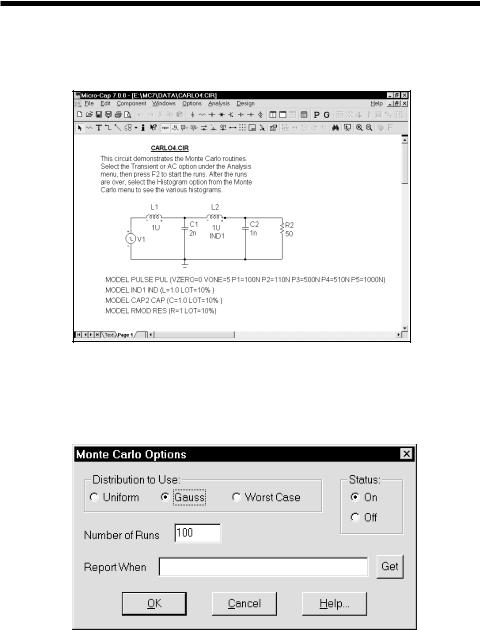
An example
To illustrate the Monte Carlo features, load the file CARLO4.CIR. This file contains a simple pulse source driving an RLC network. The circuit looks like this:
Figure 10-1 The CARLO4 circuit
Select transient analysis and then using the mouse, click the Options item from the Monte Carlo menu. It should look like this:
Figure 10-2 Monte Carlo options
189
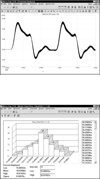
The Monte Carlo options are set to run 100 runs using a Gaussian distribution. Click on the OK button and press F2 to start the runs. The curves accumulate on the screen and the result looks like this:
Figure 10-3 The analysis run
Select Monte Carlo - Histograms - Rise_Time(V(3),1,1,1,2). This selects the existing Rise_Time histogram which looks like this:
Figure 10-4 The Rise_Time histogram
190 Chapter 10: Using Monte Carlo

This figure shows the frequency distribution for the Rise_Time performance function. The function is specified for the curve V(3), with a Boolean of 1, which selects all data points, an N value of 1 which searches for the first rise time in the V(3) curve, a Low value of 1.0, which defines the first level from which the rise time is to be measured, and a High value of 2.0, which specifies the second level from which the rise time is to be measured. The Rise_Time function measured one value from each of the 100 curves and the results are shown here in histogram form. The statistical summary at the lower left shows the lowest value, highest value, standard deviation, and mean, or average value, of the 100 numbers. The list to the right lets you scroll through individual rise time values. The Intervals value determines the number of vertical bars in the histogram. You can change the lower and upper limits in the histogram to show the percentage of the total distribution included within the limits, predicting how these limits would affect productionyields.
Now we'll add a new histogram to measure the width of the pulse. Select Monte Carlo - Histograms - Add Histogram. This presents the Properties dialog box, which you use to select a performance function. Click on the Get button and select the Width performance function. Click OK. Click OK again in the Properties dialog box a new histogram is presented.
Figure 10-5 The Width histogram
The Width function is specified for the curve V(3), with a Boolean of 1, which selects all data points, an N value of 1 which searches for the first pulse in the V(3) curve, a Level of 2.0, which defines the level at which the width of the pulse is to be measured.
191
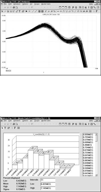
Press F3 to exit. Select AC from the Analysis menu. Press F2 and the screen should look like this:
Figure 10-6 100 plots of DB(V(3))
Select Add Histogram from the Histograms item on the Monte Carlo menu. Use the Get button to select the X_Level function for the What To Plot field. Click in the Y Level field and type -3. Click OK. Click OK again in the Properties dialog box a new histogram is presented.
Figure 10-7 AC bandwidth histogram using the X_Level function
192 Chapter 10: Using Monte Carlo
The function is specified for the curve DB(V(3)), with a Boolean of 1, which selects all data points, an N value of 1 which finds the first X value instance in the curve, a Y Level of -3.0, which defines the level at which the X value of the curve is to be measured. Since the curve is a plot of the gain of the circuit, which is a simple low pass filter, and since we chose -3 for the level, the performance function measures the 3dB bandwidth of the filter.
Press F10 to show the Properties dialog box. It includes items similar to the Plot Properties dialog boxes for the analysis plots.
Press Cancel to close the dialog box.
193

Press F3. Select DC from the Analysis menu. The Analysis Limits look like this:
Figure 10-8 The DC analysis limits
These limits specify that we plot R(R2) while stepping V1. V1 has no effect on R(R2). As a result, the plots are a series of straight lines. Press F2 to start the
Figure 10-9 A Gaussian distribution
run. Select the Peak_Y item from Monte Carlo - Histograms. The Peak_Y function measures the largest value of R(R2), which is simply the toleranced resistor value. The distribution approximates a Gaussian distribution.
194 Chapter 10: Using Monte Carlo