Micro-Cap v7.1.6 / Ug

Figure 7-14 Changing the font style of the text

Adding tags to plots

Click on the button to activate the Vertical Tag mode. Click the left mouse button near the highest peak of V(A). Drag the mouse to the highest peak of V(B) and release the button. The tag shows the vertical delta between the two data points.

Figure 7-15 Using the Vertical tag mode

145

In a similar manner, the horizontal tag, enabled by the button, measures the horizontal delta between the two data points of the tag. It is most useful for measuring the time difference between two digital events, such as the width of a pulse or the time delay between two events. Choose Delete All Objects from the Scope menu to delete the text and tag.

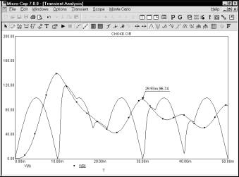
Click on the button to activate the Point Tag mode. Click the left mouse button at the second peak of V(B) and drag the mouse. The point tag labels the actual analysis data point nearest the initial mouse click. A shadow of the tag will track the mouse movements. Release the mouse button when the shadow is at the desired spot. The screen should look like Figure 7-16.

Figure 7-16 Using the Point tag

When in Select mode, double clicking on a tag element invokes the Tag dialog box. This dialog box lets you edit the arrow style, weight, color, and the font attributes of the number. All of the tag options are available for each instance of a tag element.

Both the text body and arrow tip of a tag may be repositioned after placement. Press SPACEBAR to toggle into Select mode. Double click on the tag and then deselect the Lock item in the dialog box. Click OK. Drag either the body handle or the arrow tip handle. The body handle is the small black rectangle near the text. The arrow tip handle is the small black rectangle at the tip of the tag arrow.

Press F3 to exit the analysis, then CTRL + F4 to close the file.

146 Chapter 7: Using the Scope

Performance functions

MC7 provides a group of functions for measuring performance-related curve characteristics. These functions include:

Rise_Time	This function marks the N'th time the Y expression rises
	through the specified Low and High values. It places the
	cursors at the two data points and returns the difference
	between the X expression values at these two points.
	This function is useful for measuring the rise time of
	time-domain curves.
Fall_Time	This function marks the N'th time the Y expression falls
	through the specified Low and High values. It places the
	cursors at the two data points and returns the difference
	between the X expression values at these two points.
	This function is useful for measuring the fall time of
	time-domain curves.
Peak_X	This function marks the N'th local peak of the selected
	Y expression. A peak is any data point algebraically
	larger than the neighboring data points on either side. It
	places the left or right cursor at the data point and
	returns its X expression value.
Peak_Y	This function is identical to the Peak_X function but
	returns the Y expression value. This function is useful for
	measuring overshoot in time-domain curves and the peak
	gain ripple of filters in AC analysis.
Valley_X	This function marks the N'th local valley of the selected
	Y expression. A valley is any data point algebraically
	smaller than the neighboring data points on either side. It
	places the left or right cursor at the data point and
	returns its X expression value.
Valley_Y	This function is identical to the Valley_X function but
	returns the Y expression value. It is useful for measuring
	undershoot in time-domain curves and the peak
	attenuation of filters in AC analysis.

147

	Peak_Valley	This function marks the N'th peak and N'th valley of the
		selected Y expression. It places the cursors at the two
		data points and returns the difference between the Y
		expression values at these two points. This function is
		useful for measuring ripple, overshoot, and amplitude.
	Period	The period function accurately measures the time period
		of curves by measuring the X differences between
		successive instances of the average Y value. It does this
		by first finding the average of the Y expression over the
		simulation interval where the Boolean expression is true.
		Then it searches for the N'th and N+1'th rising instance
		of the average value. The difference in the X expression
		values produces the period value. Typically a Boolean
		expression like "T>500ns" is used to exclude the errors
		introduced by the non-periodic initial transients. This
		function is useful for measuring the period of oscillators
		and voltage to frequency converters, where a curve's
		period usually needs to be measured to high precision.
	Frequency	This is the numerical complement of the Period function.
		It behaves like the Period function, but returns 1/Period.
		The function places cursors at the two data points.
	Width	This function measures the width of the Y expression
		curve by finding the N'th and N+1'th instances of the
		specified Level value. It then places cursors at the two
		data points, and returns the difference between the X
		expression values at these two points.
	High_X	This function finds the global maximum of the selected
		branch of the selected Y expression, places either the
		left or the right cursor at the data point, and returns its X
		expression value.
	High_Y	This function acts like High_X, but returns the Y value.
	Low_X	This function finds the global minimum of the selected
		branch of the selected Y expression, places either the
		left or the right cursor at the data point, and returns its X
		expression value.
148	Chapter 7: Using the Scope

Low_Y	This function acts like Low_X, but returns the Y value.
X_Level	This function finds the N'th instance of the specified Y
	Level value, places a left or right cursor there, and
	returns the X expression value.
Y_Level	This function finds the N'th instance of the specified X
	Level value, places a left or right cursor there, and
	returns the Y expression value.
X_Delta	This function finds the N'th instance of the specified Y
	expression range, places cursors at the two data points,
	and returns the difference between the X expression
	values at these two points.
Y_Delta	This function finds the N'th instance of the specified X
	expression range, places cursors at the two data points,
	and returns the difference between the Y expression
	values at these two points.
X_Range	This function finds the X range (max - min) for the N'th
	instance of the specified Y range. First it searches for the
	specified Y Low and Y High expression values. It then
	searches all data points between these two for the
	highest and lowest X values, places cursors at these two
	data points, and returns the difference between the X
	expression values at these two points. It differs from the
	X_Delta function in that it returns the difference in the
	maximum and minimum X values in the specified Y
	range, rather than the difference in the X values at the
	specified Y endpoints.
Y_Range	This function is identical to the X_Range function but it
	returns the difference in the maximum and minimum Y
	values in the specified X range This function is useful for
	measuring filter ripple.
Slope	This function finds the numeric slope at the N'th instance
	of the specified value of the X expression.
Phase_Margin	This function finds the phase margin of a curve if both
	dB(expr) and PHASE(expr) curves are plotted.

149

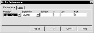
These functions may be used in performance plots, Monte Carlo analysis and 3D plotting. They may also be applied directly to single curves, which is what we will illustrate now. Load the file PERF2 and run transient analysis. When the run is

complete, click on the Go To Performance button, and drag the dialog box to the middle of the screen. The dialog box should look like this:

Figure 7-17 Go To Performance dialog box

The dialog box employs the following fields:

Function	This selects one of the performance functions.
Expression	This selects which of the expressions you want the performance
	function to perform its measurements on. Only expressions that
	were printed or plotted during the run are available.
Boolean	This expression must be true for the performance functions to
	consider a data point for inclusion in the search. Typically this
	function is used to exclude some unwanted part of the curve
	from the function search. "T>100ns" would instruct the program
	to exclude any data points for which T<=100ns.
N	This integer specifies which of the instances you want to find
	and measure. For example, there might be many pulse widths
	to measure. Number one is the first one on the left starting at
	the first time point. The value of N is incremented each time you
	click on the Go To button, measuring each succeeding instance.
Low	This field specifies the value to be used by the search routines.
	For example, in the Rise_Time function, this specifies the low
	value at which the rising edge is measured.
High	This field specifies a value to be used by the search routines.
	For example, in the Rise_Time function, this specifies the high
	value at which the rising edge is measured.

150 Chapter 7: Using the Scope

Level	This field specifies the value to be used by the search routines.
	In the Width function, for example, this specifies the expression
	value at which the width is measured.

A performance function at its core is a search. The set of data points of the target expression is searched for the criteria specified by the performance function and its parameters. All performance functions share the following general properties:

Performance functions interpolate:

Performance functions search for the closest qualifying data point and, if necessary, interpolate between it and an adjacent data point.

Performance functions find the N'th instance:

Every performance function has a parameter N which specifies which instance of the function to return. The only exceptions are the High and Low functions for which, by definition, there is a maximum of one instance.

Each performance function call increments the N parameter:

Every time a performance function is called, N is incremented after the function is called. The next call automatically finds the next instance, and moves the cursor(s) to subsequent instances. For example, each call to the Peak function locates a new peak to the right of the old peak. When the end of the curve is reached, the function rolls over to the beginning of the curve.

Only curves plotted during the run can be used:

Performance functions operate on curve data sets after the run, so only curves plotted during the run are available for analysis by a performance function.

Boolean expression must be TRUE:

Candidate data points are included only if the Boolean expression is true for the data point. The Boolean expression is provided to let the user include only the desired parts of the curve in the performance function search.

At least PERFORM_M neighboring points must qualify:

If a data point is selected, the neighboring data points must be consistent with the search criteria or the point is rejected. For example, in the peak function, a data point is considered a peak if at least PERFORM_M data points on each side have a lower Y expression value. PERFORM_M is a Global Settings value and defaults to 1. Use 2 or even 3 if the curve is particularly choppy or has any trapezoidal ringing in it.

151

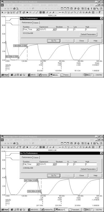
Figure 7-18 Measuring rise time

Select Rise_Time from the list box. Enter "3" in the High field and ".5" in the Low field. Enter "1" in the N field. Click on the dialog Go To button. The screen looks like Figure 7-18. N is incremented for each click of the Go To button, so successive clicks measure the rise time of successive pulses.

Select Fall_Time. Enter "1" in the N field, "3" in the High field, and ".5" in the Low field. Click the Go To button twice. The screen should look like Figure 7-19.

Figure 7-19 Measuring fall time

152 Chapter 7: Using the Scope

Select the Period function. Click on the Go To button. The screen looks like this:

Figure 7-20 Measuring the pulse period

Select the Width function and click on the Go To button. Width is computed by finding the N'th rising instance of the value Level, then the N'th falling instance of the value Level. The function returns the difference between the X expression values, and places cursors at the two locations. The screen should look like this:

Figure 7-21 Measuring the pulse width

153

Select the X_Range function. Click on Go To. The screen looks like this:

Figure 7-22 The X_Range function

X_Range locates the N'th instance of the YLow and YHigh values, places cursors at the data points and returns the difference between the X expression values. The Y_Range function works similarly. Select it and set XLow = 100n and XHigh = 200n, and click the Go To button. The result looks like this:

Figure 7-23 The Y_Range function

154 Chapter 7: Using the Scope