Micro-Cap v7.1.6 / Ug

The Uniform distribution option produces a histogram like this:

Figure 10-10 A uniform distribution

The Worst Case distribution option produces a histogram like this:

Figure 10-11 A worst case distribution

In each of the three cases, we plotted the resistance value directly, so each output histogram directly mirrored the distribution function used to determine its value.

195

The Gaussian distribution for the resistor tolerance resulted in a similar, Gaussian output distribution. For a large number of cases, the histogram closely approaches the bell shape of the standard Gaussian equation.

The uniform distribution for the resistor produced a similar uniform output distribution, although with a few bumps. If we had run a very large number of cases, we would expect a perfectly flat histogram, reflecting an equal probability of all outputs in the range.

The worst case distribution generated an output distribution that contained the two extremes. The proportion that fall into the low or high category is due to chance. The larger the number of runs, the greater the chance the proportions will be equal.

In more complex designs having many components with tolerances, the output distributions approach a standard Gaussian shape, even if the input distribution is chosen to be uniform or worst case, due to the Central Limit Theorem of statistics. It simply takes more cases to produce a normal-looking output distribution.

Press F3 to exit the analysis, and close the file with CTRL + F4.

Statistical summary

The statistical results are printed to a disk file. The file names used are:

Transient analysis	CIRCUITNAME.TMC
AC analysis	CIRCUITNAME.AMC
DC analysis	CIRCUITNAME.DMC

The content of the file may be viewed by selecting Statistics from the Monte Carlo menu when a histogram is the active window.

196 Chapter 10: Using Monte Carlo

Chapter 11 Working with Macros

What's in this chapter

This chapter describes the use of macros. The term macro is defined and the four steps of macro creation and usage are described. They are:

•

•

•

•

Creating the macro circuit file

Selecting or creating a suitable shape for the macro Entering the macro into the Component library Using the macro in a circuit

What is a macro?

Macros are complete circuits, created and saved on disk to be used as building blocks by other circuits. The principal advantage of macros is that the behavior of a complex circuit block can be incorporated into and represented by a single component. The complexity and detail of the macro is hidden from view in the calling circuit.

When an analysis is run, the macro circuit file is loaded from disk and substituted for the macro. Macro circuits are constructed in the usual way, with two exceptions.

First, macros use command text of the form,

.PARAMETERS(par1,par2,...),

to define parameters to be passed to the macro by the calling circuit.

Second, macros use grid text on circuit nodes to define the nodes (pin names) that are to be connected to the using circuit.

197

Creating the macro circuit file

The first step in using macros is to create the macro circuit itself. We won't do that here. Instead we'll use a macro circuit which is supplied with MC7. Load the macro circuit INT. It is an integrator circuit and looks like this:

Figure 11-1 The INT macro

The first stage of the macro circuit is a voltage-controlled current source (IOFV). Its transconductance value, SCALE, is passed as a numeric parameter by the calling circuit. The circuit which uses the macro is referred to as the calling circuit.

The first stage multiplies the input signal by the value SCALE and converts it to a current. The current flows directly into a capacitor, creating a voltage that is the integral of the scaled input signal. A final unity-gain stage buffers the capacitor voltage from the load in the calling circuit. The high-valued resistor avoids infinite voltages on the capacitor when DC input voltages occur. It also limits the useful range of the macro to frequencies above 1E-6, which would be acceptable for virtually all applications.

This circuit illustrates the two features which distinguish macros from ordinary circuits. First, the external pin connections are defined by placing the pin name in the form of grid text on the node where connection is desired. In the INT circuit, the text PINA, connects the positive input of the voltage-controlled current source to PINA of the macro shape. The text PINB, connects the output of the buffer stage to PINB of the macro shape.

The second important feature in this macro is that it receives parameters from the calling circuit. A macro need not have passed parameters, but most do. It can greatly enhance a macro's usefulness. The first step in passing parameters to a macro is to include the .PARAMETERS control statement in the macro circuit.

198 Chapter 11: Working with Macros

This is done by including a piece of text in the macro circuit using this format:

.PARAMETERS (<parameter[=<value>]> [, <parameter[=<value>]>]*)

The INT macro uses this particular parameters statement:

.PARAMETERS(SCALE=1,VINIT=0)

The statement defines two parameters, SCALE and VINIT. SCALE is used to multiply the input signal, and hence the integral. VINIT is used to provide an initial value to the capacitor and hence to the value of the integral.

The usual procedure is to create the INT macro circuit, then save it under the macro name. In this case it would be saved to disk under the name INT.MAC.

Selecting a suitable shape for the macro

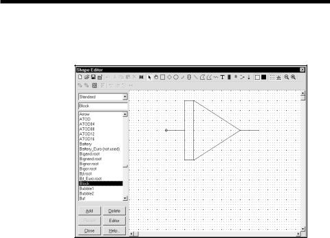
The second step in the construction of a macro is the selection or creation of a suitable shape. For our example, the Block shape will suffice. It looks like this:

Figure 11-2 The Block shape

The figure shows the Shape Editor display for the Block shape. If there are no suitable shapes in the library, you can create a new one to visually suggest the function of the macro.

199

Entering the macro into the Component library

The third step is to enter the macro in the Component library. To do this, select the Component Editor from the Windows menu. From the Component Selector, double-click on the Macros name in the Analog Primitives group. In this hierarchical selector, double-clicking opens a closed group or closes an open group.

Click on the INT name. This selects and displays the INT component. If you were adding INT as a new macro you would have clicked first on the Macro group to select it, then clicked on the Add Part button to add INT to the macro group. The INT component display looks like this:

Component selector

Shape/pin display

Attribute placement display

Figure 11-3 Component library entry for the INT macro

The Name data field is for the component name. This is the same as the macro file name. In this case we used the name INT.

The Shape data field is for the name of the shape to be used to represent the macro. The shape names are from the Shape library, which is created and maintained by the Shape editor. To select a shape, click in the Shape field and press the first letter of the shape name until the one you want appears, or use the arrow adjacent to the list to browse. Here we have chosen the Block shape.

The Definition field specifies the electrical definition. To select a definition, click in the field and press the first letter of the definition name until the one you want appears, or use the arrow to browse. In this case, we must specify Macro to indicate that the electrical definition comes from a circuit file.

200 Chapter 11: Working with Macros

The Memo field is for descriptions or comments. It has no effect on the electrical behavior of the part.

The Attribute placement display shows the location of the attribute text (XX and YY in Figure 11-3) relative to the shape. Attribute text for a macro component is comprised of the part name, macro name, and optional parameters. These are entered via the Attribute dialog box when the component is added to a schematic. You can drag the text with the left mouse button to indicate where the first (XX) and second (YY) attribute text will be initially placed. After the component is initially placed in a circuit, the attribute text can be relocated by dragging the text attribute with the mouse.

An important aspect of entering a macro into the library is defining where the pins are. For a component like a diode, the pin names are predefined as Anode and Cathode.

For a macro, pin names are defined by the user. They must match the actual node names as defined by grid text in the macro circuit.

The names are defined by clicking in the Shape / pin display field. This activates a Pin dialog box, allowing you to enter a new pin name and to specify if it is digital or analog. Double-clicking on an existing pin lets you edit it. Both the pin marker dot and the pin name can be independently dragged with the mouse to the desired locations.

201

Using the macro in a circuit

The final step is using the macro. This is the easiest part. Once the macro has been entered into the Component library, it is available for use in circuits. It is accessed from one of the groups on the Component menu.

To illustrate using a macro, we'll create a simple circuit that contains a voltage source with a sawtooth waveform driving an INT macro. The output of the INT macro should be the integral of the input waveform.

Close the Component Editor without saving any changes. Close the INT circuit. Select the New option from the File menu, then Schematic from the New dialog box. From Component Menu / Analog Primitives / Waveform Sources select the Pulse Source. Place it in the schematic with the plus sign pointing up.

Type "SAW" for the model attribute. Enter these parameters:

VZERO=-1 VONE=1 P1=0 P2=.2u P3=.2u P4=.4u P5=.4u

Click on the OK button. Click the Wire mode button. Draw a wire from the top of the pulse source to the right.

From the Macros group of the Analog Primitives section of the Component menu, select INT. Place the INT macro input at the end of the line just drawn. Type "1E7" for the SCALE parameter, and "1" for the VINIT parameter. This passes a scale value of 1E7 and an initial value of 1. Click OK. Finally, click on the Ground button in the upper tool bar, rotate it as needed with the right mouse button and place it at the minus lead of the Pulse source.

The key points about placing a macro in a circuit are:

1.Remember where you put it in the Component hierarchy. Macros are usually placed in and selected from the Analog Primitives / Macros section of the Component menu, but their location is up to you.

2.The VALUE field holds the name of the macro circuit file, such as

INT. The name must match the file name the macro circuit was saved under. 3. Each parameter is entered as a separate attribute.

202 Chapter 11: Working with Macros

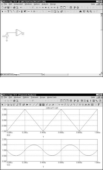
The final circuit and its transient analysis are shown in the figures below. To produce this analysis you must disable the operating point and change the plot scales in the analysis limits dialog box.

Figure 11-4 The INT macro used in a circuit

Figure 11-5 Transient analysis of the circuit

Press F3, and close the circuit.

203

An easy way to create macros

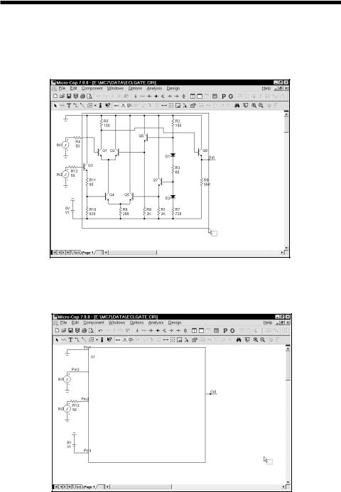
Another way to make macros from existing circuits is to use the macro creation command. To illustrate, load the file ECLGATE. Enter Select mode, and drag a box region across the circuit like this:

Figure 11-6 The ECLGATE macro box region

Be sure to draw the box region exactly as shown above. Now press CTRL + M. Click OK in the dialog box. The screen should look like this:

Figure 11-7 The ECLGATE circuit using a macro

204 Chapter 11: Working with Macros