Micro-Cap v7.1.6 / Ug

An AC example

How about AC? The basic operation is the same, but there are differences. To illustrate the differences, press F3 to exit Probe and unload the ECLGATE circuit. Load the file DIFFAMP. Select Probe AC from the Analysis menu. Click on the Vertical menu. It looks like this:

Figure 8-5 AC Probe variables and operators

The list of variables includes the usual voltage and current variables, but excludes charge, capacitance, flux, inductance, B, H, and time. There are several new variables; INOISE, ONOISE, and frequency. Additionally, the complex math operators, Magnitude, Magnitude (dB), Phase (PH), Group Delay (GD), Real Part (RE), and Imag Part (IM) are available. The short form is shown in parentheses. One of these operators is always selected. When you choose a circuit variable by clicking in the schematic, the selected operator is applied to the circuit variable and the result plotted. Magnitude is the default operator. For example, V(10) is the magnitude of V(10). PH(V(10)) is the phase of V(10). As in normal AC analysis, the noise variables can not be mixed with other variables, such as voltage or current.

Click on the dot near the node labeled A. Using the right mouse button, pan the schematic to the left by dragging in the schematic. Pan until the right portion of the diffamp is visible. Click on the dot near the node labeled OutA. Click on the

Cursor mode button to enable the Cursor mode. The results should look like Figure 8-6.

165

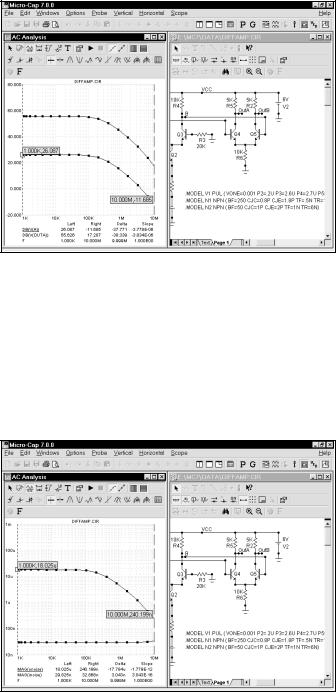
Figure 8-6 Reading AC gains using the Cursor mode

The left plot cursor is initially placed at the first data point, 1Khz. The low frequency gain at the two nodes A and OutA can be read out directly under the Left column. Use the left mouse button to move the left cursor to obtain additional readings. The right plot cursor is controlled by the right mouse button.

Press CTRL + F9. Select Magnitude, Log, and ONOISE from the Vertical menu and click anywhere in the schematic. Select INOISE from the Vertical menu and click anywhere in the schematic. This plots input and output noise:

Figure 8-7 AC noise plots

166 Chapter 8: Using Probe

A DC example

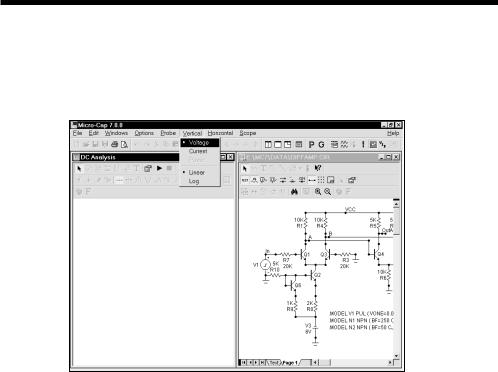
We'll use the file DIFFAMP to illustrate the use of Probe in DC. Exit the AC Probe routine by pressing F3. Select Probe DC from the Analysis menu. Click on the Vertical menu. It looks like this:

Figure 8-8 DC Probe variables

The list of available vertical variables includes voltage, current, and power. The horizontal variable is initially the voltage across the Input1 source when you start or press CTRL + F9 to clear the curves. The horizontal variable can be changed after the first curve has been placed by first selecting the plot window, and then pressing F10 to invoke the Characteristics dialog box. Simply type in a new expression into the Plot X field.

Press ESC to remove the Vertical menu.

Click on the dot near the node labeled OutA. Using the right mouse button, pan the schematic to the left by dragging in the schematic. Pan until the right portion of the diffamp is visible. Click on the dot near the node labeled 'OutB'. Click on

the Cursor button to enable Cursor mode. The results should look like Figure 8-9.

167

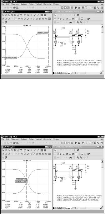
Figure 8-9 DC transfer function plot

Click on the Inflection button. This moves the left plot cursor to the next inflection point to the right of its current position (first data point). Press SHIFT + LEFT ARROW key. This moves the right plot cursor to the next inflection point to the left of its current position (last data point). The peak gain 603, which occurs near the inflection point, can be read out directly in the Slope column. The inflection mode is useful for determining the peak DC gain of an amplifier.

Figure 8-10 Using the cursors to find the peak gain

168 Chapter 8: Using Probe

Probing a SPICE file

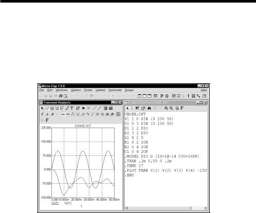
MC7 can also probe SPICE files. Exit DC Probe with F3 and load CHOKE.CKT. Select Analysis / Probe Transient. MC7 presents the Analysis Limits dialog box to let you change the run conditions if you want. Press ESC to remove the dialog box and click on the text V1 and again on C1. MC7 plots the voltage across the V1 source and the C1 capacitor.

Figure 8-11 Probing SPICE circuits

Clicking on two-terminal devices like sources, resistors, diodes, and the like plots the voltage across or current through the device, depending upon whether the Vertical option is set to Voltage or Current.

Clicking on three-terminal devices, presents a dialog box where you can select the desired voltage or current variable.

Clicking on a node number plots the node voltage.

169

170 Chapter 8: Using Probe

Chapter 9 Stepping Component Parameters

What's in this chapter

Stepping is the process of systematically changing one or more numeric parameters to see what effect the parameter(s) may have on circuit behavior. You can step simple parameters, like a resistor's value, or a model statement parameter like the forward beta of a transistor, or a symbolic parameter.

In this chapter, we demonstrate how to use stepping with several tutorials. The topics include:

•How parameter stepping works

•Stepping in transient analysis

•AC and DC examples

•Stepping summary

171

How parameter stepping works

Stepping and Monte Carlo are mutually exclusive. Only one may be active at a time.

Stepping systematically alters the value of one or more parameters of one or more components and then runs the analysis, drawing multiple branches for each curve. Most parameter types can be stepped, including component parameters like the resistance of a resistor, model parameters like a transistor beta, and symbolic parameters created with a .define or .param command. If the parameter changes the equation matrix, MC7 simply recreates the equations. For each parameter set, a run is made and the specified curves plotted.

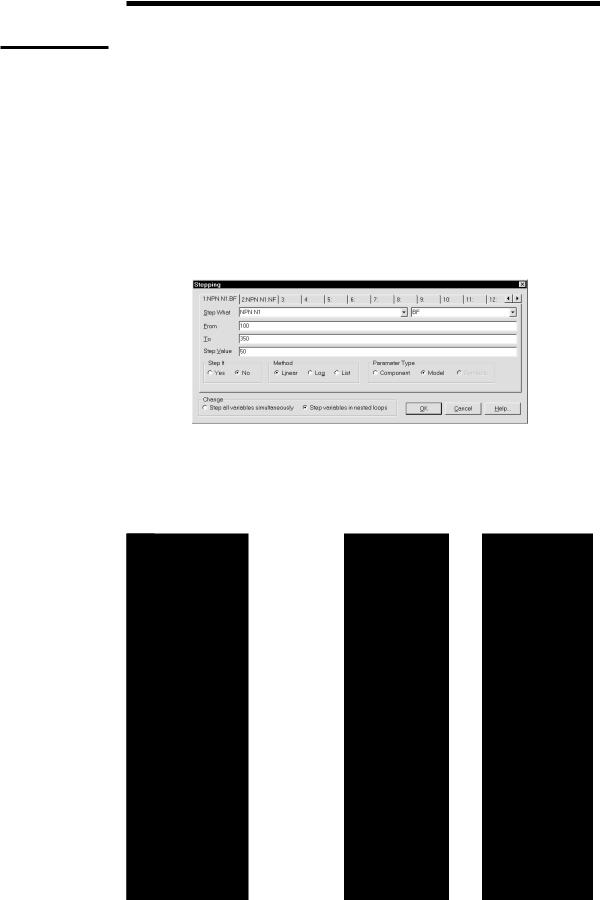
To illustrate stepping, load the circuit DIFFAMP. Select Transient from the Analysis menu. Press F11, click on the Stepping button in the Analysis Limits dialog box, or click on the Stepping button to display the Stepping dialog box. It looks like this:

Figure 9-1 The Stepping dialog box

The dialog box provides tabs for up to twenty parameters, although two or three is a practical maximum. Each tab accesses a panel which controls a single parameter. Stepping for each parameter is enabled when its Step It option is set to Yes.

The left Step What list box specifies the name of the model whose parameter is to be stepped. Since dissimilar parts may share the same model name, the electrical definition is shown along with the name. This can be seen in Figure 9-1 where the first item is NPN N1. This specifies that we want to step one of the parameters of all bipolar NPN transistors using the model name N1. Clicking on the list box arrow displays a list of the models available for stepping. To select a model, click on it.

The right Step What list box specifies the name of the model parameter to be

172 Chapter 9: Stepping Component Parameters

stepped. Clicking on the list box arrow displays a list of the parameters available for stepping. To select a particular parameter, click on it. In this case we want to step the BF (forward beta) parameter, so leave it as it is.

The From field in each panel specifies the starting value of the parameter for the first run. The To field specifies the ending value of the parameter for the last run. The Step Value field specifies how much the parameter changes between steps.

The Method option in each panel controls how the Step Value affects the parameter value. Linear stepping adds the Step Value to the parameter value. Log stepping multiplies the parameter by the Step Value. List stepping lets you enter a comma-delimited set of specific values in the From field.

The Parameter Type option in each panel specifies whether the Step What field refers to a model name, component name, or symbolic name. You can step an individual instance of a model parameter or all instances of the model parameter. If the Type option is set to Model, all instances are simultaneously stepped. If this option is set to Component and the PRIVATEANALOG / PRIVATEDIGITAL (Options / Global Settings) flags are enabled, then only the instance whose component name matches the Step What field will have its parameter stepped.

The Change option only comes into play when stepping multiple parameters. It controls whether the parameter changes are to be nested or simultaneous. For example, suppose you step R1 through the values 10 and 20. Suppose also that you step C2 through the values 1n and 5n. Simultaneous stepping will generate two runs and nested stepping will produce four runs as shown below.

Nested	Simultaneous
R1=10 C2=1n	R1=10 C2=1n
R1=10 C2=5n	R1=20 C2=5n
R1=20 C2=1n
R1=20 C2=5n

Simultaneous stepping requires an equal number of steps for each parameter. Use nested stepping when you want all combinations of parameter variation. Use simultaneous stepping when you want only specific combinations.

173

Stepping in transient analysis

To see how stepping works in transient analysis, click the Yes button in Parameter panel 1, click OK, and press F2 to start the run. It looks like this:

Figure 9-2 Stepping BF in four transistors simultaneously

In this run, each device which uses the N1 model, which includes the transistors Q1, Q3, Q4, and Q5, has its BF (forward beta) stepped through the values 100, 150, ... 350. To see which devices use N1, double-click on each device in the schematic to see its Attribute dialog box. From the results, it seems the offset voltage of V(OUTA,OUTB) is insensitive to large changes in BF, if all four devices have the same value.

Now we'll step the BF of just Q1 to see how the circuit tolerates small relative differences in beta. Press F11 to access the Stepping dialog box. Click on the Component item in the Parameter Type group. From the Step What list, click on Q1 and from the parameter list select BF. Type "250" in the From field, "255" in the To field, and "1" in the Step Value field. Click on the OK button and press F2 to start the run. The plot, shown in Figure 9-3, demonstrates the circuit sensitivity to differential beta. When Q1's BF changes from 250 to 255, while all other transistors have constant BF, large shifts occur in the output offset of both curves V(A,B) and V(OUTA,OUTB).

174 Chapter 9: Stepping Component Parameters