Micro-Cap v7.1.6 / Ug

•Value Format: This accesses a dialog box where you select the numeric format used to print the X value in the cursor table and in the tracker boxes.

•Auto Scale: This command scales the X Range and places the numbers into the Low, High, and Interval fields. The effect on the plot can be seen by clicking the Apply button.

•Log: If checked this makes the scale log.

•Y: This group provides corresponding commands for the Y axis group:

•Range Low: This is the low value of the Y range used to plot the selected curve.

•Range High: This is the high value of the Y range used to plot the selected curve.

•Grid Spacing: This is the distance between Y grids.

•Bold Grid Spacing: This is the distance between bold Y grids.

•Scale Format: This is the numeric format used to print the Y axis scale.

•Value Format: This accesses a dialog box where you select the numeric format used to print the Y value in the cursor table and in the tracker boxes.

•Auto Scale: This command scales the Y Range and places the numbers into the Range Low, Range High, and Interval fields. The effect on the plot can be seen by clicking the Apply button.

•Log: If checked this makes the scale log.

•Same Y Scales: If enabled, Auto Scale determines a single common scale for all curves within a plot group. If the box is unchecked, the Auto Scale command determines individual scales for each curve.

•Save Range Edits: Enabling this check box causes any edits to the range fields to be copied to the appropriate range fields of the Analysis Limits dialog box, making them permanent.

95

Slope Calculation: This lets you pick Standard, dB/Octave, or dB/Decade method of calculating slopes. The latter two are useful in AC analysis.

Use Common Formats: Clicking this button copies the X and Y formats of the selected curve to the format fields of all curves.

•Colors, Fonts, and Lines

•Objects: This list box lets you select the object that the other group controls apply to. Objects include:

•General Text: This is text used for axis scales, titles, cursor tables, and curve names.

•Grid: This is the analysis plot grid.

•Graph Background: This is the plot background.

•Window Background: This is the window background.

•Select: This is the Select mode.

•Select Box: This is the Select mode box.

•Initial Object: This governs the initial properties of analysis text, graphical objects, and numeric tags. Object properties can be changed after they are added to a plot by double-clicking on them in Select mode.

•Tracker: This controls the visual properties such as color and font of the numeric cursor trackers.

•Select Color Primary: This sets the color of the curve that the left cursor is on when there is more than one branch.

•Select Color Secondary: This sets the color of the curve that the right cursor is on when there is more than one branch and the two cursors are on different branches.

•Data Point Labels: This controls the visual properties such as color and font of the data point labels.

96 Chapter 4: Transient Analysis

• Curve Names: This controls the visual properties of the lines and text used to display each curve. "Plot All" lets you set properties for all curves simultaneously.

•Object Names (Color): This group lets you change the foreground and background color and other object characteristics of selected objects.

•Font: This group lets you change the font of the selected object.

•Size: This group lets you change the text size of the selected object.

•Style: This group lets you change the text style of the selected object.

•Effects: This group lets you change text effects of the selected object.

•Sample: This group shows a sample curve line using currently selected color, width, and pattern properties.

•Header: This group controls the header format for text numeric output.

•Left: This group lets you add text to the left side of the text output.

•Center: This group lets you add text to the center of the text output.

•Right: This group lets you add text to the right side of the text output. In each case the following formats are available:

$MC	Prints Micro-Cap
$User	Prints user name
$Company	Prints company name
$Analysis	Print analysis type (Transient, AC, DC)
$Name	Prints circuit name

You can use these or any other text in the left, center, or right.

• Delimiters: This group lets you select the delimiter that will be placed between items in the text output. The choices are Tab, Semicolon, Comma, Space, or Other.

• Save Curves: This group lets you save one or more curves for later display in a plot or use in a User source. It provides these fields:

97

•Curves: This lets you select the curve that the other fields apply to.

•Temperature: If the analysis run stepped temperature and produced multiple curves this field lets you select which to save.

•Stepped Variable: If the analysis run stepped a variable and produced multiple curves, this field lets you select which to save.

•Save Curve: This field is a copy of the selected curve name.

•As (New Name): This field lets you specify the curve's name. It is the name you use later to display or use the curve in a source.

•In File: This field specifies the file name for the curve.

•Save: This command saves the selected curve using the specified curve name and file name. Note that when curves are saved to existing files, they are added to the file. If the curve already exists in the file, it is overwritten. All other curves in the file are unaffected.

•Browse: This command lets you browse directories for the file name you want to save the curve under or to delete.

•Delete: This command lets you delete the specified curve.

•Tool Bar: This page lets you select the buttons that will appear in the local tool bar area below the Main tool bar.

The four buttons at the bottom have the following function:

•OK: This button accepts all changes, exits the dialog box, and redraws the analysis plot. Subsequent runs will use the changed properties and they will be retained in the circuit file, if the file itself is later saved.

•Cancel: This button rejects all changes, exits the dialog box, and redraws the analysis plot using the original properties.

•Apply: This button redraws the analysis plot using the current settings in the dialog box to show how the display would be affected by the changes. The changes are still tentative, until the OK button is clicked.

•Help: This displays the help information for the Plot Properties dialog box.

98 Chapter 4: Transient Analysis

Data Points

Option

Let's experiment with some of the other options. Click on the Data Points button . This toggles the display of marker icons for the calculated data points. Since

the option was initially disabled, clicking the button enables it, and the data point marker icons are added producing a plot that looks like this:

Figure 4-8 The plot with the Data Points option enabled

Since the simulator uses a variable time step algorithm to minimize errors and accelerate the run, the actual time points will not be regularly spaced. The data point markers are placed at the actual computed time points. There are at least two situations where you might want to see these:

Inadequate curve sampling: This can happen in transient analysis when the simulator flies past a switch threshold. It may also happen that you want more data points to "fill in" source curves that look choppy. Even though the charge error is strictly controlled by the internal truncation error routines, the data sampling may seem inadequate. Data point icons show where the data points are and whether more will help. In AC analysis, your plot may miss a steep spike on a narrow pass or reject band. Data point icons show whether the simulator actually made a calculation within the band.

Identifying real curve spikes: Sometimes you see spikes on curves. If the curve changes direction from one data point to the next, it's likely the spikes are simply artifacts of the integration routines. The only way to tell is to mark the data points. If they are integration artifacts, you can reduce them by decreasing RELTOL or the minimum time step or both.

99

Experimenting	To illustrate some other options, click on the horizontal axis grid		and vertical
	axis grid	buttons. The plot should now look like this:
with the options

Figure 4-9 Adding grids to the plot

Press F9, then click on the Operating Point and Operating Point Only buttons. This tells the program to do an operating point calculation, and then stop. An operating point calculation sets all sources to their defined initial values, removes all capacitors, and replaces all inductors with short circuits. It then calculates the steady-state DC values of the state variables (node voltages, inductor currents and digital states) at the initial time point. This set of values is referred to as the DC operating point. Press F2 to do the operating point only run. Since we're doing only an operating point, no plot will appear. Exit the analysis by pressing F3. Click on the Node Voltage button and MC7 displays the last calculated states and voltages. In this case, since we just completed an operating point only calculation, these are the operating point values.

100 Chapter 4: Transient Analysis

State variables and initialization

State variables are the variables that uniquely define the state of the circuit. These include node voltages, inductor currents, and digital node states. MC7 determines the initial state variable values according to the following rules:

When you first select transient analysis, MC7 sets all state variables to zero and all digital levels to X. This is called the setup initialization.

Each time you start a new run, with F2 or clicking the Run button, MC7 does the run initialization. To decide what to do, it looks at the State Variables option from the Analysis Limits dialog box. There are three choices:

Zero: Node voltages and inductor currents are set to 0. Digital levels are set to X, or in the case of flip-flop Q and QB outputs, to 0, 1, or X depending upon the value of the global variable DIGINITSTATE. This value is accessed from Options / Global Settings.

Read: MC7 reads the variables from the file CIRCUITNAME.TOP. The file is created by the State Variables editor Write command.

Leave: MC7 does nothing to the state variables. It simply leaves them alone. There are three possibilities:

First run: If the variables have not been edited with the State Variables editor, they still retain the setup initialization values.

Later run: If the variables have not been changed by the State Variables editor, they retain the ending values from the last run.

Edited: If the variables have been changed by the State

Variables editor, they are the values shown in the editor.

The states of all nodes connected to digital stimulus sources are changed to the T=0 value. Using these initial values, an optional operating point calculation may be done. If an operating point is done, the state variables are, of course, changed accordingly. If an operating point is not done, the state variables at the first (T=0) time point are used as initial conditions for starting the run, but interpolated backwards from the second and third time points after the run is over. If the Operating Point Only option is enabled, the analysis ends after the operating point calculation and the final state variable values are the DC operating point values.

101

The State Variables editor

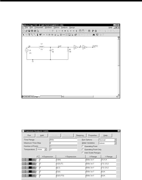
To illustrate the State Variables editor load the circuit, MIXED1. It looks like this:

Figure 4-10 The MIXED1 circuit

This circuit contains an analog section driving a digital section. Select Transient from the Analysis menu. The analysis limits look like this:

Figure 4-11 The MIXED1 analysis limits

102 Chapter 4: Transient Analysis

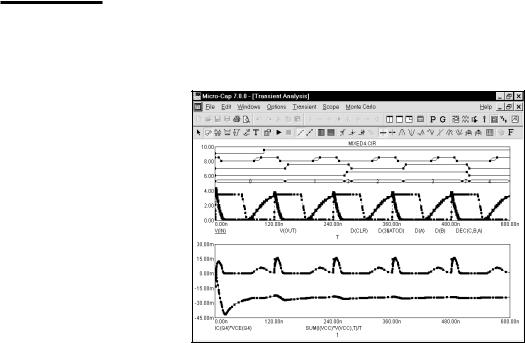
Press F2 to start the run. The results look like this:

Figure 4-12 The transient analysis run

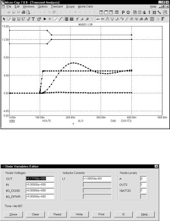
Select the State Variables Editor from the Transient menu. It looks like this:

Figure 4-13 The State Variables editor

This editor lets you view and edit state variable values. State variables consist of node voltages, shown in the left column, inductor currents, shown in the middle column, and digital node levels, shown in the right column. Node voltages and digital node levels are identified by the node name, if one exists, or the node number otherwise. Inductors are identified by the part name.

The display shows the current values of the state variables. Since we've just finished a transient analysis these values are from the last data point of the run.

Let's experiment with these values. Double-click the mouse in the L1 inductor field and type ".2". This sets the inductor current to 0.2 amps. Double-click in the OUT voltage field and type "6". This sets the OUT node to 6.0 volts. Double-click

103

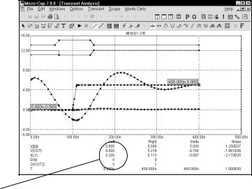
in the OUT2 digital node level field and type "X". This sets the OUT2 node level to X. Click on the Close button. The Run Options from the Analysis Limits dialog box are set to skip the operating point and to leave the state variables when we start the run. These choices tell the program to use the current state variables values, which we have just edited, for the initial values. Since we have requested no operating point, the initial point on the plot should reflect the values in the State Variables editor. Press F2 to start the run. When the run is complete, press F8 to place the display in the Cursor mode. The results look like this:

Initial values

Figure 4-14 The new run in Cursor mode

Notice that the initial value of V(OUT) (shown under the Left cursor column), is the 6.0 volts we specified in the State Variables editor. Similarly, the initial value of the inductor current is 0.2 and the initial value of the digital level of node OUT2 is X.

Exit the analysis with F3 and close the circuit file with CTRL + F4.

104 Chapter 4: Transient Analysis