Micro-Cap v7.1.6 / Ug

Chapter 5

AC analysis

What's in this chapter

AC analysis is the topic for this tutorial. In particular, these subjects are covered:

•AC analysis

•The AC Analysis Limits dialog box

•Experimenting with the options and limits

•Selecting curves to plot or print

•Picking plot options

•Numeric output

•Input and output noise plots

•Nyquist plots

•Smith charts

•Polar plots

105

AC analysis

What happens during an AC analysis? First, an optional DC operating point is calculated. Digital nodes stabilize at an operating point state and potentially affect analog nodes to which they may be attached. Linearized, small signal AC models are then created for each component and integrated into a set of linear network equations. These are repeatedly solved at many frequency points to obtain the small signal response of the circuit to whatever AC excitation is present in the circuit. The linearized AC model of a digital component is an open circuit. This means that digital parts are ignored during small signal analysis.

The excitation is supplied by one or more independent curve sources in the circuit. Pulse and Sine sources provide a fixed, real, 1.0 volt AC signal. User sources provide a signal comprised of the real and imaginary parts specified in their files. The SPICE independent sources, V and I, provide user-specified real AC signal amplitudes. Function sources can create an AC signal only if they have a FREQ expression. These are the only sources that generate AC excitation.

AC analysis represents the excitation and system variables (node voltages and various branch currents) as complex quantities. Operators, such as RE (real), IM (imaginary), dB (20*Log()), MAG (magnitude), PH (phase), and GD (group delay) are provided to print and plot these complex quantities.

To explore AC analysis, load the file DIFFAMP. It looks like this:

Figure 5-1 The DIFFAMP circuit

106 Chapter 5: AC Analysis

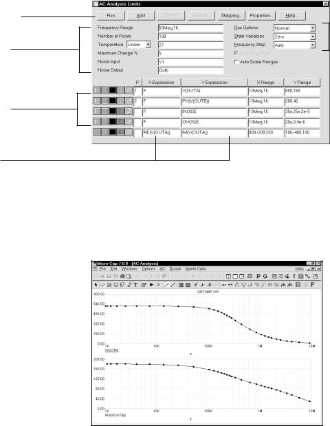
Choose AC from the Analysis menu. When the AC Analysis Limits dialog box comes up, the fields should look like this:

Command buttons

Options

Numeric limits

Curve options

Expressions

Figure 5-2 The AC Analysis Limits dialog box

In this circuit, we have a single source providing a 1.0 volt AC signal. The dialog box instructs MC7 to sweep the frequency from 1K to 10Meg and produce plots of the magnitude of the voltage at the node OUTA and the phase angle of the voltage at node OUTB. Press F2 and the result looks like this:

Figure 5-3 The AC analysis plot

107

Command buttons

Numeric limits

The AC Analysis Limits dialog box

The Analysis Limits dialog box is divided into five principal areas: the Command buttons, Numeric limits, Curve options, Expressions, and Options.

The command buttons are located just above the Numeric limits.

Run: This command starts the analysis run. Clicking the Tool bar Run button or pressing F2 will also start the run.

Add: This command adds another Curve options field and Expression

field line after the line containing the cursor. The scroll bar to the right of the Expression field scrolls the curve rows when needed.

Delete: This command deletes the Curve option field and Expression field line where the text cursor is.

Expand: This command expands the working area for the text field where the text cursor currently is. A dialog box is provided for editing or viewing. To use the feature, click in an expression field, then click the Expand button.

Stepping: This command calls up the Stepping dialog box. Stepping is reviewed in a separate chapter.

Properties: This command invokes the Properties dialog box which lets you control the analysis plot window and the way curves are displayed. See

the Plot Properties dialog box article in Chapter 4, "Transient Analysis".

Help: This command calls up the Help Screen. The Help System provides information by index and topic.

The definition of each item in the Numeric limits field is as follows:

•Frequency Range: This field controls the frequency range for the analysis. The syntax is <Highest Frequency> [, <Lowest Frequency>]. If <Lowest Frequency> is unspecified, the program calculates a single data point at <Highest Frequency>.

•Number of Points: This determines the number of data points printed in the Numeric Output window. It also determines the number of data points

108 Chapter 5: AC Analysis

actually calculated if Linear or Log stepping is used. If the Auto Step method is selected, the number of points actually calculated is controlled by the <Maximum change %> value. If Auto is selected, interpolation is used to produce the specified number of points. The default value is 51. This number is usually set to an odd value to produce an even print interval.

For the Linear method, the frequency step and the print interval are:

(<Highest Frequency> - <Lowest Frequency>)/(<Number of points> - 1)

For the Log method, the frequency step and the print interval are:

(<Highest Frequency> / <Lowest Frequency>)1/(<Number of points> - 1)

• Temperature: This field controls the temperature of the run. If the Temperature list box shows Linear the format is:

<high> [ , <low> [ , <step> ] ]

The default value of <low> is <high>, and the default value of <step> is <high> - <low>.

If the Temperature list box shows List the format is:

<t1> [ , <t2> [ , <t3> ] [ ,...]]

where t1, t2,.. are individual values of temperature.

All values are in degrees Celsius. One analysis is done at each specified temperature, producing one set of curves for each.

•Maximum Change %: This value controls the frequency step used when Auto is selected for the Frequency Step method.

•Noise Input: This is the name of the input source to be used for noise calculations. If the INOISE and ONOISE variables are not used in the expression fields, this field is ignored.

•Noise Output: This field holds the name(s) or number(s) of the output node(s) to be used for noise calculations. If the INOISE and ONOISE variables are not used in the expression fields, this field is ignored.

109

Curve options

Expressions

The Curve options are located below the Numeric limits and to the left of the Expressions. Each curve option affects only the curve in its row. The options function as follows:

The first option toggles the X-axis between a linear and a log plot. Log plots require positive scale ranges.

The second option toggles the Y-axis between a linear and a log plot. Log plots require positive scale ranges.

The option activates the color menu. There are 64 color choices for an individual curve. The button color is the curve color.

The option prints a table showing the numeric value of the curve.

The values printed are those actually calculated. The table is printed to the Numeric Output window and saved in the file CIRCUITNAME.ANO.

The option selects the basic plot type. In AC analysis there are three types available, rectangular, polar, and Smith.

A number from 1 to 9 in the P column is used to group the curves into different plot groups. All curves with like numbers are placed in the same plot group. If the P column is blank, the curve is not plotted.

The Expressions field specifies the horizontal (X) and vertical (Y) scale ranges and expressions. The expressions are treated as complex quantities. Some common expressions are F (frequency), db(v(1)) (voltage in decibels at node 1), and re(v(1)) (real voltage at node 1). Note that while the expressions are evaluated as complex quantities, only the magnitude of the Y expression vs. the magnitude of the X expression is plotted. If you plot the expression V(3)/V(2), MC7 evaluates the expression as a complex quantity, then plots the magnitude of the final result. It is not possible to plot a complex quantity directly vs. frequency. You can plot the imaginary part of an expression vs. its real part (a Nyquist plot), or you can plot the magnitude, real, or imaginary parts vs. frequency (a Bode plot).

The scale ranges specify the scales to use when plotting the X and Y expressions. The range format is:

<high> [,<low>] [,<grid spacing>] [,<bold grid spacing>]

110 Chapter 5: AC Analysis

<low> defaults to zero. [,<grid spacing>] sets the spacing between grids. [,<bold grid spacing>] sets the spacing between bold grids. Placing "AUTO" in the X or Y scale range calculates its range automatically. The Auto Scale Ranges option calculates scales for all ranges during the simulation run and updates the X and Y Range fields. The Auto Scale (F6) command immediately scales all curves, without changing the range values, letting you restore them with CTRL + HOME if desired. Note that <grid spacing> and <bold grid spacing> are used only on linear scales. Logarithmic scales use a natural grid spacing of 1/10 the major grid values and bold is not used. The Auto Scale command uses the Preferences / Auto Scale Grids value to set the grid spacing if none is specified in the range.

Clicking the right mouse button in the Y expression field invokes the Variables list. It lets you select variables, constants, functions, and operators, or expand the field to allow editing long expressions. Clicking the right mouse button in the other fields invokes a simpler menu showing suitable choices.

• Run Options

Options

•Normal: This runs the simulation without saving it to disk.

•Save: This runs the simulation and saves it to disk in the Probe format.

•Retrieve: This loads a previously saved simulation and plots and prints it as if it were a new run.

•State Variables: These options determine what happens to the time domain state variables (DC voltages, currents, and digital states) prior to the optional operating point.

•Zero: This sets the state variable initial values (node voltages, inductor currents, digital states) to zero or X. This option forces an operating point.

•Read: This reads a previously saved set of state variables and uses them as the initial values for the run. Normally the values read in are from a prior operating point run in AC or transient analysis, and are the desired bias conditions about which to linearize and do the AC analysis. If so, you would want to disable the Operating Point option when you use this Read feature. This option forces an operating point.

•Leave: This leaves the current values of state variables alone. They retain their last values. If this is the first run, they are zero. If you have

111

just run an analysis without returning to the Schematic editor, they are the values from that run. This option does not force an operating point.

•Frequency step

•Auto: This method uses the first plot of the first group as a pilot plot. If, from one frequency point to another, the plot has a vertical change of greater than [maximum change %] of full scale, the frequency step is reduced, otherwise it is increased. [maximum change %] is the value from the fourth numeric field of the AC Analysis Limits dialog box. Auto is the standard method because it uses the fewest number of data points to produce the smoothest plot.

•Linear: This method uses a frequency step that produces horizontally equidistant data points on a linear scale. The number of data points is controlled by the Number of Points field.

•Log: This method uses a frequency step that produces horizontally equidistant data points on a log scale. The number of data points is controlled by the Number of Points field.

•List: This method uses a comma-delimited list of frequency points from the Frequency Range, as in 1E8, 1E7, 5E6.

•Operating Point: This calculates a DC operating point, changing the state variables as a result. If an operating point is not done, the time domain variables are those resulting from the initialization step (zero, leave, or read). The linearization for AC analysis is done using the state variables after this optional operating point. In a nonlinear circuit where no operating point is done, the validity of the small-signal analysis depends upon the accuracy of the state variables read from disk, edited manually, or enforced by device initial values or .IC statements. Calculating an operating point may (and usually does) change the initial state variables.

•Auto Scale Ranges: This sets all ranges to Auto every time a simulation is run. If disabled, the values from the range fields are used.

All options affect simulation results. To see their effect, you must do a run by clicking on the Run command button.

112 Chapter 5: AC Analysis

Experimenting with options and limits

The small squares on the plots in Figure 5-3 mark the actual points calculated by MC7. We can produce a smoother plot at the expense of more data points by reducing the Maximum change % value from 5% to 1%. Display the AC Analysis Limits dialog box with F9. Double-click the mouse in the Maximum Change % field and type "1". Press F2 to run the analysis. It looks like this:

Figure 5-4 The plot with Maximum change % set to 1%

The lower value of 1% produces a smoother plot by calculating more data points. The current Frequency Step method is Auto. In this mode, the frequency step is automatically adjusted to restrain the point-to-point change of both the vertical value and the angle of the plot itself to less than the specified maximum change. The Auto method produces the smoothest plot at the lowest computation price for most curves.

This analysis uses 1% and generates about three times the number of data points as the 5% analysis. Since the analysis time increases in direct proportion to the number of data points, it is wise to keep the Maximum change % as large as possible. A value of 1 to 5 is usually suitable. If the first curve is very flat, you may want to try a fixed frequency step method.

Let's try one of these methods. Press F9 to display the Analysis Limits dialog box. Click in the Frequency Step list box. When the list drops down, click on the Log option. Press F2 to start the run. The result looks like Figure 5-5.

113

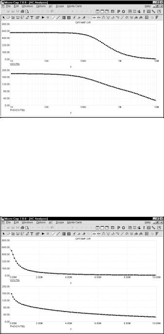
Figure 5-5 The plot using the log option

The constant horizontal distance between data points is achieved by making each new frequency a product of the prior frequency and a fixed multiplier. Since the lowest frequency forms the base that is multiplied, it must not be zero.

The Linear option is only used when the X axis is linear. To illustrate, press F9 and edit the Frequency Range field to 1E7,0. Change the Frequency Step method to Linear and change the X Log/Linear button states of the first two curves to linear. Press F2 to run. The result looks like Figure 5-6.

Figure 5-6 The plot using the linear option

114 Chapter 5: AC Analysis