Micro-Cap v7.1.6 / Ug

Chapter 14 Using Animation Mode

What's in this chapter

Animation mode is an alternative way of visualizing analysis results. It performs the selected analysis and plots any specified waveform. While it is plotting, it is also updating any animation devices on the schematic along with any on-sche- matic display values. In this chapter, we demonstrate Animation mode's capability with an example. The topics include:

•How Animation mode works

•Animation components

•Animate Options dialog box

•A Transient example

225

How Animation mode works

Animation mode is another way to view simulation results. In this mode, a single analysis data point is taken and the on-schematic display values and animation components are updated on the schematic. Micro-Cap then waits for either a key press or a specified time delay before calculating the next data point. The purpose is to slow the simulation down to be able to monitor the updated changes on the schematic. The on-schematic display values let the node voltages, branch currents, power dissipation, and device conditions of the latest data point be viewed on the schematic. The animation components that update are the digital switch, LED, and seven segment display. While primarily designed to operate in transient analysis with digital components, this mode is available in transient, AC, and DC with any type of circuit.

In transient analysis, a single time step is calculated, and any on-schematic display values or animation components are updated on the schematic. When a key is pressed or after the specified delay time has elapsed, the solution at a new time point is calculated and the schematic updated accordingly. The schematic always displays the values from the last time step calculated.

In AC analysis, the schematic displays the on-schematic display values and states of the animation components from the operating point calculation. These values are fixed during the entire simulation. Even though the schematic displays are fixed at the operating point, the animation mode will calculate a single frequency data point when a key has been pressed or the specified time delay has elapsed.

In DC analysis, a single DC sweep data point is calculated, and any on-schematic display values or animation components are updated on the schematic. When a key is pressed or after the specified delay time has elapsed, the next DC sweep data point is calculated and the schematic updated accordingly. The schematic always displays the values from the last DC sweep data point calculated.

226 Chapter 14: Using Animation Mode

Animation components

There are three animation components: a digital switch, an LED, and a seven segment display. The description of these are as follows:

Digital Switch: The switch is designed to produce either a digital zero or one state. It has a single output pin at which the selected digital state will appear. During a simulation, the switch may be clicked on to toggle it between its zero and one output. The appearance of the switch's arm will change to indicate which state the switch is currently connected to.

LED: The LED component is designed to represent the display of a light emitting diode. It has a single input pin. Depending on the digital state or the analog voltage at the input pin, the LED will be lit with a different color on the schematic. The colors the LED uses are defined in the Color/Font page of the circuit's Properties dialog box. In this page, there is a list of digital states that have a corresponding color.

Seven Segment Display: The seven segment component is designed to represent the display of a seven segment display. It has an input pin for each segment of the display. All of the pins are active high. It is intended to work with basic seven segment decoders/drivers although any input will control the display of the corresponding segment.

The LED and seven segment display components do not model the electrical characteristics of the parts they represent. They are only available for display purposes. The digital switch is the only one of the three that can affect a simulation. Each of these components must have an I/O model specified for them in order to work with analog components.

227

Animate Options dialog box

This dialog box sets the interval between data point calculations in an animation analysis. The dialog box is invoked by selecting Animate Options under the Scope menu and appears in Figure 14-1. It provides these options:

Wait

Don't Wait: This option turns off the animation which lets the analysis run at optimum speed.

Wait for Key Press: This option will produce one data point with each key press.

Wait for Time Delay: This option will produce one data point per specified time delay.

Time Delay: This text field sets the specified time delay in seconds that will be between each data point calculation. This text field is only active if the Wait for Time Delay option is selected.

OK: This closes the dialog box and saves any changes that were made.

Cancel: This closes the dialog box and ignores any changes that were made.

Help: This accesses the help topic for this dialog box.

Figure 14-1 Animate Options dialog box

228 Chapter 14: Using Animation Mode

A transient analysis example

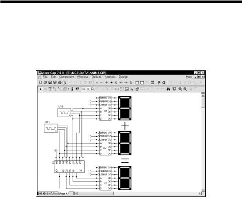
To see how the animation mode works in transient analysis, click on Open under the File menu and load the circuit ANIM3. The ANIM3 circuit uses the seven segment components to display the outputs of three 7448 seven segment decoders. The circuit should appear like this:

Figure 14-2 The ANIM3 circuit

Select Transient from the Analysis menu. Close the Analysis Limits dialog box. Click on the Scope menu and select Animate Options. The Wait setting for the ANIM3 circuit is currently set to Wait for Time Delay and the Time Delay has been defined as 0.5. This means that a single data point will be calculated every half second. Click OK. Hit the F2 key to run the simulation. The resulting values will be displayed in the plot and on the schematic. Notice that both the digital states on the schematic and the seven segment displays are updated with each data point. Figures 14-3 and 14-4 display the simulation results at two separate times in the circuit.

For animate mode, a split screen should be used to be able to view both the waveform plot and the schematic at the same time. This can be done by selecting Tile Vertical or Tile Horizontal under the Windows menu. The schematic can be moved within the window by dragging with the right mouse button.

229

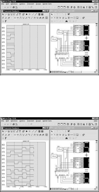
Figure 14-3 Animation mode results at 200ns

The waveforms in the plot also show the output values of the Ina stimulus (nodes 21-18), the Inb stimulus (nodes 28-25), and the resulting output (nodes 35-32) of the adder. As can be easily seen in the figures, it is much easier to view the basic output through the animation components than through the actual waveforms.

Figure 14-4 Animation mode results at 700ns

230 Chapter 14: Using Animation Mode

	Symbols
Index
	$MAXPAGE			217
	$MAXSHEET			217
	.SUBCKT	211
	3D plots	43
	A
	AC analysis		105
	Accessing			46, 107
	Excitation			106
	System variables						106
	Accel PCB interface						26
	Active filters			48
	Add page command						29
	Add Part wizard				53
	Add Parts wizard				213
	Adding components						62, 82
	Adding tags to plots						145
	Adding text to plots						144
	Align cursors command							133
	Analog library			32
	Analog primitives					32,		66
	Analog waveforms						8, 16
	Analysis Limits dialog
	box	8,	84, 108,					123,		124
	Command buttons
	Add	84,		108, 124
	Delete		84,		108,			124
	Expand			85, 108,				124
	Help	85, 108,					124
	Properties				85
	Run	84,		108,			124
	Stepping			85,		108, 124
	Numeric limits field
	Frequency range							108
	Maximum change %								109
	Maximum time step								85
	Noise input				109
	Noise output					109
	Number of points							85, 108, 126
	Temperature				85, 109, 125
	Time range				85
	Options
	Auto scale ranges							88,		112, 128

Frequency step						112
Normal run					87, 111, 128
Operating point						88,	112
Operating point only							88
Retrieve run					87, 111,			128
Save run				87, 111, 128
State variables options
Leave		88, 111
Read		88,		111
Zero		87, 111
Animation		50, 156, 225
Components				227
Example		229
Mode	33, 225
Options		228
Arrange icons command							34
Attributes		19,		30,		62
Dialog box				62, 71, 72
Text	20
Text display command							38
Auto scale command						131
Auto scale option					87, 111,			127
B
B field plots			159
Baseline	131
Batch mode		17
Behavioral modeling						1
Bessel filters				48
Border display command							38
Bottom cursor position mode								139
Box 19, 29
Bring to front command							30
BSIM models				1
C
Calculator		35
Capacitance plots					159
Cascade command						34
Characteristic plot command								64
Charge plots			159
Chebyshev filters					48
Clear command				28, 73
Clear cut wire command							28

231

Click the mouse	19
Clipboard 19
Close command	27
Color command	30

Color menu		86, 110, 127
Command line			17
Command line operation 17
Component
Definition		19
Menu	32
Component Editor
Access command 35
Add group command					53
Add part command					53
Add Part wizard				53
Adding a new component						51
Assign command				52
Clear Palette command						54
Creating pins			21
Display	51
Display Value / Model Name							52
Export to MC6 command						53
Find command				54
Import wizard			53
Info command			54
Merge command				53
Move command				54
New file command					53
Open file command					53
Parts list command					53
Paste command				54
Pin assignments				52
Pin text option				52
Redo command				54
Replace command					54
Sort command				54
Undo command				54
User palette assignment						52
User palette membership						65
Component library				1
Component mode command						36
Condition display command						38
Copy command			19, 28, 74, 82
Copy to clipboard command						28
Copy to picture file command							29

Cross-hair display command								38
Current		7,	160
Current display command 38
Cursor		19
Cursor mode				13,		134, 137, 138
Cursor mode command							37
Cursor value fields						137
Cut command				28, 73, 82
D
Data directory				4
Data entry			25
DC analysis			46
Default component						82
Default setting for new circuits									42
Define command					6
Delete all objects command								131
Delete page command							29
Deleting objects					73
Demos		49
Deselecting objects						75
Design menu				48
DEV tolerances					184
Dialog boxes				25
Digital
Hex operator					7
State		7
Digital library				32
Digital primitives						32,	66
Digital waveforms						8,	16
Drag	19
Drag copying				76, 82
DSP	50
Dynamic DC analysis							12, 46,		50
E
Edit menu			28
Editing parameters and text								71
Elliptic filters				48
Equipment required						3
Esc key		20
Exit command				27
Expressions			8, 13, 89

232

F

File
Binary model				56
Text model			56
File menu		26
New command				26
Open command				26
Save as command					26
Save command				26
Filter designer			50
Filters	33, 48
Find command			31
Find component command							33
Flag mode command					37
Flip X command				29
Flip Y command				29
Font command			30
Fourier analysis				50
Function keys			58
CTRL + F11 Optimizer						58
CTRL + F4 Close window								58
CTRL + F6 Change window								58
CTRL + F9 Delete all plots								58
F1 Help		58
F10 Properties dialog box								58
F11 Stepping dialog box							58
F12 State Variables editor								58
F2 Run analysis				58
F3 Exit analysis				58
F4 Display analysis plot							58
F5 Display numeric output								58
F6 Auto scale				58
F7 Scale mode				58
F8 Cursor mode					58
F9 Analysis Limits dialog box 58
G
Gaussian distribution					186
Global settings			45,		173
Gmin stepping			40
Graphics mode command						36
Grid	20
Grid text		20
Grid text display command							38

H

H field plots 159 Hardware requirements 3 Help mode command 37 Help System 49 Horizontal tag mode 134

Horizontal tag mode command 37

I

I-V characteristics 123 Import wizard 53 Inductance plots 159 Inertial cancellation 40 Info mode command 37 Initialization 101 INOISE 116 Installation 4

Inverse-Chebyshev filters 48

K

Key ID 49

L

Linear DC stepping 125

Linear plot option 86

List DC stepping 125

Load MC file 27

Log DC stepping 125

Log plot option 86

LOT 184

LOT tolerances 184

M

Macro

Definition 20, 197 Parameters command 198

Maximize command 34 Maximum time step 85 MC6 5

Menus 22 Selection 24

Mirror box command 29

233

Mode commands	36	Node voltages display command 38
Model Editor		Noise
Add command	57	Analysis	116
Copy command	57	Flicker	116
Delete command 57		Shot 116

Go to command				57				Thermal			116
Memo field			57					NOM.LIB			208, 212
Merge command					57			Normalize command							132
Pack command				57				Number of points						85, 108,			126
Part field		57						Numeric output
Part selector			57					AC	115
Type Selector				57				DC	126
Model editor			56					Transient			85
Model library			56					Nyquist plots				118
Binary form			56					O
Text form		56
MODEL program				5, 35, 56				Object	21
Monte Carlo
								ONOISE		116
Distributions
								Open model file					56
Gaussian			186
								Optimizer			14
Uniform			186
								Optimizer demo					50
Worst case				186
								OrCad PCB interface							26
Example		189
								P
How it works 184
Options								P column		8
Distribution to Use						188
Number of Runs					188			Package editor					35
Report When				188				PADS PCB interface							26
Status		188						Page	29
Standard deviation					186			Scroll bar controls							23
Monte Carlo analysis					50			Selector tabs					23
N								Panning		21,		79,		136, 164
								Passive filters					48
Navigating		77, 82, 164						Paste command					21,		28, 73,		74, 82
								PCB interface					1, 26,			35
Paging	77
								Performance functions								1, 147,		187
Panning		77
								Performance plots						50
Relocation			77
								Picture	29
New command			82
								Picture files				71
Node
								Pin assignments					52
Definition			20
								Pin connections					67
Names	20, 69, 82
								Pin connections display command										38
Numbers		21, 69
								Pin definition					21
Node number assignment						69
								Plot group number						86
Node numbers display command							38
								Plotting waveforms							7,	89
Node snap		70

234