Micro-Cap v7.1.6 / Ug

Chapter 2 Exploring the Basics

What's in this chapter

This chapter covers the basics of operating the program. It presumes that you are familiar with the Windows user interface and shows you how Micro-Cap employs that interface to create and analyze electronic circuits. The chapter also reviews the key terms and concepts central to the operation of the program.

Program structure

Micro-Cap 7 includes two executable programs:

• MC7	This is the main program.
• MODEL	This is the modeling program.

MC7, the main program, provides the seamless integration of creation, analysis, and display tools for which the Micro-Cap family is famous.

MODEL is an auxiliary program designed to make the creation of device models from data sheet parameters fast, easy, and accurate. It includes an interactive, optimizing curve fitter that takes data points from graphs or tables and produces an optimized set of model parameters. MODEL can be run from the Program Manager and from within MC7.

How to start MC7

Micro-Cap 7 is activated in the usual way if Windows is already active, by double-clicking on its icon.

Before you run Micro-Cap 7, insert the security key into one of the parallel ports. The key must be connected to a parallel port to start MC7 and must remain there while running the program. If you are using the LAN version, the red LAN key should be in the server parallel port.

5

A quick tour

As a quick introduction to MC7, we'll take a brief tour of the program. Begin with a double click on the MC7 icon.

To begin the tour, we'll load one of the sample circuit files supplied with MC7. Choose Open from the File menu. When the file prompt comes up, type in the file name "MIXED4". Click Open. The program loads the circuit and displays it.

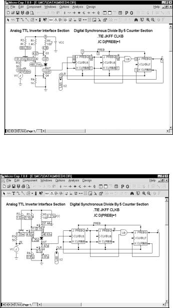
Figure 2-1 The MIXED4 sample circuit

The circuit uses an analog TTL inverter to drive a digital three-stage synchronous divide-by-five counter. The digital clock input to the first JK flip-flop is driven by the analog TTL output, while the CLR initializing pulse for the flip-flops comes from a digital source, U2. The CLK inputs are connected together with a .TIE command. The flip-flop preset nodes are connected together by a wire and the node is labeled PREB with grid text. This node is initialized to a '1' state with an

.IC command. The digital source states are specified in a .DEFINE command statement located in the schematic text area. The text area is a private cache in each schematic for storing text. You can toggle the display between the drawing and text areas by pressing CTRL + G or by clicking on the Text tab in the lower page scroll bar. This combination of analog and digital circuitry is easily handled by the program, since it contains a native, event-driven digital simulation engine, internally synchronized with its SPICE-based analog simulation engine. MicroCap 7 is a true mixed-signal simulator.

6 Chapter 2: Exploring The Basics

Transient analysisdisplay

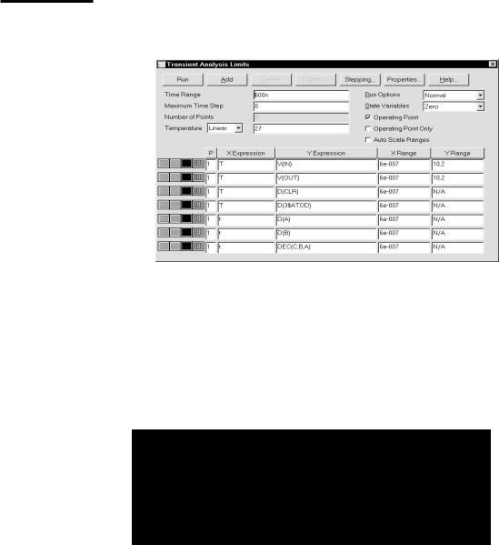
Select Transient from the Analysis menu. MC7 presents the Analysis Limits dialog box where you specify the simulation time range, choose plot and simulation options, and select waveforms to be plotted during the run.

Figure 2-2 The Analysis Limits dialog box

Here we have chosen to plot the analog voltage waveforms at the input pulse source, the output of the analog section, and several of the digital waveforms. In general, MC7 can plot any expression using as variables any node voltage or state or any device terminal voltage or current. Here are a few other expressions that could have been plotted in this circuit.

	d(CLR)	Digital state waveform on node CLR.
	hex(CLR,PB,1,2)	Hex waveform at nodes CLR,PB,1,2.
	vbe(q3)	Base-emitter voltage of transistor q3.
	I(VCC)	Current through the VCC source.
	PG(VCC)	Power generated by the VCC source.
	qbe(q1)	Charge stored in the base-emitter cap of q1.
	cbc(q4)	Base-collector capacitance of q4.

There are a great many other variables available for plotting. Click the right mouse button in the Y Expression field to see a list of variables available for plotting or printing. Click outside of the menu to remove it.

7

Now let's run the actual simulation. Click on the Run button or press F2 to start the simulation. MC7 plots the results during the run. The run can be stopped at any time by clicking the Stop button , or by pressing ESC.

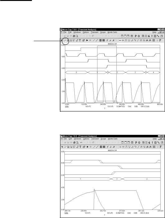
Figure 2-3 Transient analysis of the circuit

The final waveform plots look like Figure 2-3. Each waveform can have a unique token, width, pattern, and color. These options are set from Options / Default Properties for New Circuits for new circuits and can be changed for the current circuit from the Properties (F10) dialog box. Waveforms can be grouped into one or more plots. Grouping is controlled by the plot number assigned to each waveform. The plot number is the number in the P column of the Analysis Limits dialog box. You can assign all the waveforms to a single plot, or group them into as many plots as will fit on the screen. To assign several waveforms to the same plot, give them all the same plot number. To create several plots, use different plot numbers. To disable plotting a waveform, enter a blank for the plot number.

In this example, all waveforms in the plot group share a common vertical scale. You can use different scales by disabling the Scope / Same Y Scales option and specifying the scales you want in the Y Range field. All waveforms in a plot group always share the same horizontal or X scale.

Digital and analog waveforms may be mixed or separated. Separated digital waveforms show the expression on the left, adjacent to the plot. Mixed digital waveforms display the expression at the bottom of the plot along with the analog expressions in the order of their occurrence in the Analysis Limits dialog box.

8 Chapter 2: Exploring The Basics

Zooming in on a waveform

Place the mouse near the top middle of the waveform plot group. Press the left mouse button and while holding it down, slide the mouse down and to the right to create an outline box as shown in the figure below. Release the mouse button and MC7 magnifies and redraws the box region.

You must be in Scale mode to zoom in with the mouse.

Figure 2-4 Using the mouse to magnify a waveform

If you make a mistake, press CTRL + HOME and try again.

Figure 2-5 The magnified region

9

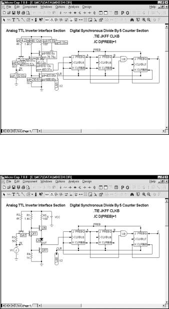
Press F3 to quit the analysis. Select Dynamic DC from the Analysis menu. This runs a DC operating point and displays the node voltages and digital states like this:

Figure 2-6 Operating point node voltages and states

Click to turn off voltages and click to display currents like this:

Figure 2-7 Operating point DC currents

10 Chapter 2: Exploring The Basics

Click to turn off currents and click to display power terms like this:

Figure 2-8 Operating point DC power terms

Click to turn off power and click to display conditions like this:

Figure 2-9 Operating point DC conditions

The voltage, current, power, and condition are the current time-domain values, which in this case is the result of a DC operating point calculation.

11

Turn off the Dynamic DC analysis mode from the Analysis menu. Remove the AC analysis MIXED4 circuit by choosing Close from the File menu. Load a new file by

choosing Open from the File menu. Type RCA3040 for the name. Click Open.

Figure 2-10 The RCA3040 circuit

Select AC from the Analysis menu. As before, an analysis limits dialog box appears. We have chosen to plot the voltage of the two nodes, Out1 and Out2, in dB. Click on the Run button, and the analysis plot looks like this:

Figure 2-11 AC analysis plot

12 Chapter 2: Exploring The Basics

Scope in Cursor mode

The same rich set of expressions available in transient analysis is also available in AC analysis. In addition, these operators are very useful:

		db(c)	Finds the decibel value of the complex expression c.
		re(c)	Finds the real value of the complex expression c.
		im(c)	Finds the imaginary value of the complex expression c.
		ph(c)	Finds the phase in degrees of the complex expression c.
		gd(c)	Finds the group delay of the complex expression c.
		inoise	Finds the input noise reflected to the input node.
		onoise	Finds the output noise at the output node.

Click on the Cursor mode button in the Tool bar or press F8. In this mode, two cursors are placed on the graph and may be moved about. The table below the plots show the waveform values at each of the two cursors, the difference between them, and the slope. The display should look like this:

Right cursor tracker

Left cursor tracker

Figure 2-12 Cursor mode

The left mouse button controls the left cursor and the right button controls the right cursor. The cursor keys LEFT ARROW and RIGHT ARROW also control the cursors. As the cursors move around, the numeric display continuously updates to show the value of the waveforms, the change in waveforms between the two cursors, and the waveform slope between the two cursors. The optional cursor trackers also track the X and Y values as the cursors are moved.

13

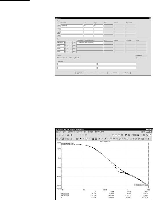
Note from Fig 2-10 that the load resistors R1 and R3 are set to RL, a symbolic The Optimizer variable defined as 1.32K. We'll optimize the value of RL to maximize the gain at

1MHz. Press CTRL + F11 to bring up the Optimizer. It looks like this:

Figure 2-13 The Optimizer dialog box

These settings seek the value of RL that maximizes the performance function Y_Level(DB(V(OUT1)),1,1,1E6). From Fig 2-12 the value of DB(V(OUT1)) at 1.0Mhz before optimization is 40.9dB. Click on the Optimize button. The optimizer whirs and chugs and eventually spits out an optimal value of 2.3K. Click on the Apply and Close buttons. Press F2 to rerun the analysis, then F8 and you'll see that with RL=2.3K, DB(V(OUT1)) at 1Mhz is now 45.4dB, a net gain of 4.5dB. Press F3 to exit the AC analysis routine. Choose Close from the File menu to unload the circuit.

Figure 2-14 The optimized gain curve

14 Chapter 2: Exploring The Basics