Micro-Cap v7.1.6 / Ug

Magnifying

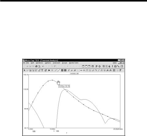
Press ESC twice to remove the menus. Click the left mouse button just above and to the left of the large peak of the V(B) curve. While holding the left button down, drag the mouse down and to the right to create a magnification box like the one shown in Figure 7-3.

Figure 7-3 Magnifying a region

Release the button and MC7 scales the plot to match the outline of the box.

Figure 7-4 The magnified region

135

Panning

Panning is like scrolling in a text field, except that it is multidirectional. To illustrate, click the right mouse button in the middle of the plot. The mouse arrow cursor changes to a hand cursor. While holding the right button down, drag the mouse slowly up and to the left until it nearly touches the upper left corner of the plot window. The effect is like sliding a paper across a desk. Dragging the mouse dynamically updates the display to reflect the change in view. Release the button and the plot looks like this:

Figure 7-5 Panning the plot

As with panning in the Schematic editor, the keyboard may also be used. The CTRL key plus the arrow keys move the view in the direction of the arrow.

The combination of panning and magnifying allows close inspection of any portion of the curves.

Note that you can also scale (magnify) and pan while in Cursor mode:

Scaling:	CTRL + left mouse drag
Panning:	CTRL + right mouse drag

Press CTRL + HOME or choose Restore Limit Scales from the Scope menu to return the analysis to its original offset and scale.

136 Chapter 7: Using the Scope

Cursor mode

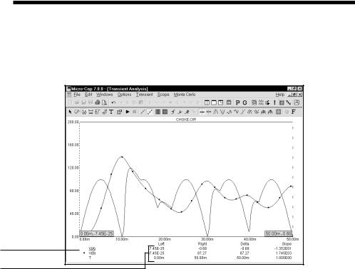
Click on the Cursor mode button or Press F8 to place Scope in the Cursor mode. In this mode the display looks like this:

Selected curve

Cursor value fields

Figure 7-6 The Cursor mode

The Cursor value fields, located below the plots, show the numeric value of each curve or expression at both cursor positions. The X expression value is shown below the Y expression values. The purpose of each field is as follows:

•Left: This shows the value of the row's Y expression at the left cursor.

•Right: This shows the value of the row's Y expression at the right cursor.

•Delta: This shows the value of the row's Y expression at the right cursor minus the value of the Y expression at the left cursor.

•Slope: This shows the row's Y expression delta value divided by the delta value of the X expression. If the X expression is T (time), then this field approximates the time derivative of the curve between the two cursors. The slope calculation can be changed to dB/Octave or dB/Decade from Properties / Scales and Formats, if dB is used in the Y expression and F (frequency) is the X expression.

137

Cursor mode panning and scaling

Mouse

Normal mouse-controlled scaling and panning are not available in Cursor mode, since the mouse movements in this mode are used to control the left and right curve cursors. However, by using the CTRL key together with the mouse, you can pan and scale within Cursor mode as follows:

Scaling:	CTRL + left mouse drag
Panning:	CTRL + right mouse drag.

To scale (magnify) the curves, press the CTRL key down and drag with the left mouse button.

To pan the curves, press the CTRL key down and drag with the right mouse button.

Keyboard

To pan the curves with the keyboard, press the CTRL key down and press the LEFT ARROW or RIGHT ARROW keys.

There is no keyboard-based scaling procedure.

138 Chapter 7: Using the Scope

Cursor mode positioning

Drag with the left mouse button to control the left cursor, and the right button to control the right cursor. The LEFT ARROW and RIGHT ARROW cursor keys move the left cursor and SHIFT + cursor keys move the right cursor. The mouse places the cursor anywhere, even between simulation data points. The keyboard moves the cursor to one of the simulation data points, depending on the positioning mode. The positioning mode, chosen with a Tool bar button, affects where the cursor is placed the next time a cursor key is pressed. Cursor positioning picks locations on the selected, or underlined, curve. Curves are selected with the Tab key, or by clicking the Y expression with the mouse.

•Next Simulation Data Point: In this mode, pressing the cursor keys finds the next actual data point in the direction of the cursor arrow from the run.

•Next Interpolated Data Point: In this mode, pressing the cursor keys finds the next rounded interpolated data point in the direction of the cursor arrow.

•Peak: In this mode, pressing the cursor keys finds the next local peak on the selected curve.

•Valley: In this mode, pressing the cursor keys finds the next local valley on the selected curve.

•High: Clicking this button finds the data point with the largest algebraic value on the current branch of the selected curve.

•Low: Clicking this button finds the data point with the smallest algebraic value on the current branch of the selected curve.

•Inflection: In this mode, pressing the cursor keys finds the next data point with the largest magnitude of slope, or first derivative, on the selected curve.

•Top: Clicking this button finds the data point with the greatest Y value of all branches of the selected curve at the current X cursor position.

•Bottom: Clicking this button finds the data point with the smallest Y value of all branches of the selected curve at the current X cursor position.

139

•Global High: Clicking this button finds the data point with the largest algebraic Y value of all data points on all branches of the selected curve.

•Global Low: Clicking this button finds the data point with the smallest algebraic Y value of all data points on all branches of the selected curve.

When Cursor mode is selected, a few initialization events occur. The selected curve is set to the first, or top curve. The Next mode is enabled. Clicking on a mode button not only changes the mode, it also moves the last cursor in the last direction. The last cursor is set to the left cursor and the last direction is set to the right. The left cursor is placed at the left on the first data point. The right cursor is placed at the right on the last data point.

140 Chapter 7: Using the Scope

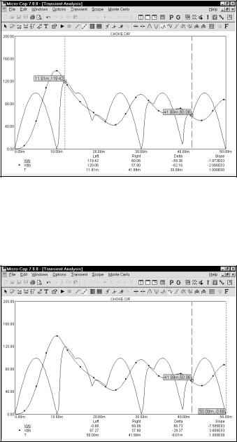
Click on the Peak button. The left cursor moves to the first peak to the right of its current position on the selected curve, V(A). Press SHIFT + LEFT ARROW key. The right cursor moves to the first peak on its left.

Figure 7-7 Using the Peak mode

Click on the button to select the Valley mode. Press the RIGHT ARROW key. The cursors are placed on the next valley in the right and left directions.

Figure 7-8 Using the Valley mode

141

Click on the High button. The left cursor moves to the global high on the selected curve.

Figure 7-9 Using the High mode

Click on the button to select the Low mode. The left cursor is positioned at the right hand edge of the plot, the global low for the curve.

Figure 7-10 Using the Low mode

142 Chapter 7: Using the Scope

Click on the Inflection button. The left cursor moves to the next inflection point on the selected curve. Press SHIFT + RIGHT ARROW key. The right cursor moves to the next inflection point on the selected curve moving right to left.

Figure 7-11 Using the Inflection mode

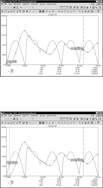
Click on the Go to Y button. Type "50" in the dialog box that comes up and click on the 'Left' button in the dialog box. The left cursor is positioned at the first incidence of 50.0 for the selected curve's Y expression value.

Figure 7-12 Using the Go to Y mode

143

Adding text to plots

Adding text to an analysis plot is easy. Click on the Close button to exit the Go

To Y mode. Click on the button to select the Text mode. Click the mouse near the large peak of the V(B) curve and type "V(B) peaks at 138 volts.". Click OK. The screen looks like this:

Figure 7-13 Adding text to a plot

Would the text look better if it were centered over the peak? To see if it would, first enter Select mode by pressing the SPACEBAR or by clicking on the Select

button . Next, click on the text with the left button and drag it to the left until it is centered. Release the button and the text is redrawn at the mouse position.

Perhaps the text would look better if it were bold. Double click on the text and when the text dialog box is presented, click on the Font tab in the dialog box. This part of the dialog box lets you change the font and several font attributes. In this case, we need to change the Style attribute. From the Font Style group, select the Bold option. Click on the OK button. The text should now appear as in Figure 7- 14. All font attributes for each instance of text are independently changeable.

144 Chapter 7: Using the Scope