Emerging Tools for Single-Cell Analysis

Fluidics and Optics

27

F i g . 2.3. Interval distribution of unrelated events. The mean event rate is µ events per second.

illuminated by the laser light while traveling a distance of the spot plus the cell diameter. When two events are in the illumination spot at the same time, the instrument is likely to have trouble accurately determining the properties of each cell individually. To avoid erroneous classification of cells, the incidence of double occupancy should be kept low. Coincident events, which may cause measurement errors, should be at least an order of magnitude lower than single events. Poisson again serves as a guideline (Fig. 2.1). The average beam occupancy (cycle time) should be below 0.1. Even then, a significant fraction of measurements (again about 0.1) will be affected by coincident events. In uncertain measurement conditions, the instrument should not sort. Therefore, the circuitry should detect coincident events and flag the measurement so that these events can be rejected for sorting by the downstream charge circuitry.

FLUIDICS AND OPTICS

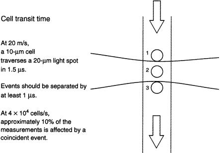
The considerations of the maximum analysis rate lead to the following specifications for the optical and fluid path design. Cells are about 10 µm in diameter. In order to fully illuminate a cell, the laser spot must be somewhat larger. A well-collimated laser and a diffraction-limited lens with a focal length of 100 mm generate a spot about 20 µm in diameter. A jet propelled by 60 psi (1 psi = 0.07 kg/cm2) moves at ~20 m/s, yielding a cell transit time of ~1.5 µs. Furthermore, some time is needed for the electronics to return to the baseline conditions, a minimum of 1 s. An illumination duty cycle of 0.1 corresponds to a maximum event rate of 40,000 events/s.

28	High-Speed Cell Sorting

F i g . 2.4. Cell diameter and transit time.

A spot size of 20 µm and fluid pressures of 100 psi or less can be obtained with generally available technology. In a balanced system, the electronic modules must be capable of an analysis rate (and therefore a maximum sort rate) of at least a few 10,000 cells/s. A further increase in speed requires a smaller spot size or a higher jet velocity. A smaller spot size will result in partial illumination of the particle and consequently requires much more complex electronics to obtain an accurate measurement. Higher jet velocities require a significantly higher sheath pressure, complicating the fluid delivery systems. We will limit the current discussion to systems analyzing at 40,000 events/s.

The foregoing identifies the cell transit time as a rate-limiting factor. The importance of the transit time has interesting consequences for sorter design that are not generally appreciated. First, in order to achieve stable jet formation, the pressure drop across the nozzle orifice must be large. Therefore, the velocity of the jet is always considerably faster than the fluid flow in the other parts of the system. Consequently, cuvette systems, in which the cells are measured before they accelerate into the jet, are at least an order of magnitude slower than jet-in-air systems. Second, the number of photons that can be collected from a particle are, to a first approximation, proportional to the illumination time. Short transit times reduce the number of photons collected and therefore the sensitivity. This reduction in photon emission may be compensated to some extent by increasing the illumination intensity (van den Engh and Farmer, 1992). High-speed sorters therefore typically require more powerful lasers than do slow systems.

Electronics

29

ELECTRONICS

Electronic circuits accept the signals from the photodetectors (usually photomultipliers), condition the signals, perform analog-to-digital conversion, collate the digital information for event classification, and, after checking for coincident events, issue sort commands for those cells that fall within specified sort windows. The circuits must perform these tasks without affecting the overall speed of sorting.

Experiments with high-speed sorters often search for cells that occur at a very low incidence in the starting sample. In many cases, the unique identification of such rare cells requires determination of a large number of cell characteristics. Throughout the years, the number of fluorescence signals that is considered routine has increased steadily. Recently, Herzenberg’s group reported the use of 11 fluorescent tags with 3 excitation lasers for the isolation of hemopoietic progenitor cells (Baumgarth et al., 1998). Even when a limited set of parameters is sufficient to uniquely describe the cell of interest, inclusion of additional parameters may be beneficial. All measurement systems make mistakes occasionally. Erroneous measurements may be confused with a sortable event, leading to sort contamination. In rare-cell sorting, measurement artifacts may become a significant factor. By increasing the number of criteria (parameters) that define a sortable event, we can reduce the chance of an identification error leading to a sorted event. The measurement of redundant properties increases the overall accuracy of our experiments. The electronics for a high-speed sorter should be capable of processing as many parameters as we wish to measure.

High-speed sorters generate fluorescence pulses that are 1–2 µs in width, limiting the average event rate to about 40,000 events/s. The electronic modules should not further constrain this speed. Ideally, the pulse-processing electronics are capable of measuring and digitizing the events with a cycle time of 3 µs or less. The downstream digital acquisition and classification circuits must be able to deal with at least 16 parameters, or 180 ns per parameter. A well-behaved acquisition and event-processing system capable of handling asynchronous events at such speeds requires careful design (van den Engh and Stokdijk, 1989).

A simple test may be performed to determine the cycle time of sorter electronics. A periodic pulse with the duration of a typical fluorescence pulse is offered to the signal amplifiers. The sort windows are set such that all pulses result in a sorted event. Starting at a low repetition rate, the frequency of the pulse generator is gradually increased. At a low rate, the trigger rate and the sort rate will be the same as the frequency of the presented signals. At some point there will be a discrepancy between the number of pulses offered and the number of pulses processed. This frequency marks the cycle time of the instrument.

Two events arriving within one cycle time of each other may not be processed correctly and may lead to measurement errors. The two events are processed as if they represent a single occurrence. The properties reported are a hybrid of the properties of the two original particles. This artifact is known as a correlation error. Suppose we have one cell with fluorescence intensities x1 and y2, followed closely by another cell with properties x2 and y1 (Fig. 2.5). A correlation error may cause the recording of a nonexistent cell with a signature x2, y2. Immunologists might interpret the

30	High-Speed Cell Sorting

F i g . 2.5. Correlation errors create ghost events. A sample contains two cell types with fluorescent properties x1, y2 and x2, y1. Two cells that occupy the illumination spot simultaneously may generate the erroneous measurement x2, y2, artificially creating a “rare double-positive cell.” If a cell population is located orthogonally to two main populations, correlation errors should be considered. The relative frequency of ghost events depends on the cell analysis rate.

measurement error as a double-positive cell. Sorting of events with such properties will deliver a mixed population—both cells will be represented—in which a variety of biological functions may be found. Correlation errors often resemble clusters of rare events at orthogonal positions in a bivariate fluorescence plot. Great care should be exercised when such clusters are selected for sorting. One test for the occurrence of correlation errors is to run a sample at varying rates. If the number of events in an orthogonal cluster is rate dependent, chances are that it represents an electronic artifact rather than a real cell population.

It will be clear that high-speed, multiparameter operation of sorters severely tests the quality of the electronic circuitry. Researchers performing experiments in which purity or accuracy is crucial should check carefully for artifacts. One way to test the error rate of the acquisition electronics is to operate the system near full duty cycle. This test may be done by activating the main trigger circuit with a high-frequency stochastic signal, for instance from a photomultiplier registering dim ambient light or by

Drop Generation

31

passing a dense bead suspension through the flow cytometer at a rapid rate. The trigger rate must be such that a significant number of events fall within the cycle time of the instrument. The channels that are not attached to the trigger circuit should sample a simple signal with known characteristics, such as a sine wave from a function generator. Despite the high trigger rate, the measurements should yield plots that are consistent with the simple signals that are offered to the acquisition system. For example, the recorded data, when plotted as a time series, should reconstruct a perfect sine wave or a Lissajoux figure. Sometimes errors happen only at a very precise moment in the trigger cycle, for instance when a second pulse coincides exactly with the transition of a digital component somewhere in the system. When such critical timing conditions are suspected, two digital pulses with a sliding time separation can be offered to the system. By varying the time between the two pulses, the conditions of the rare error can be forced to happen at a higher frequency.

Considering the foregoing, it should be clear that the electronics should be fairly fast for reliable high-speed sorting. Although the speed of even the most advanced cell sorter is modest in terms of modern electronic integrated circuits, a sorter combines many electronic functions that need to work in concert. The asynchronous nature of the events makes error conditions virtually unavoidable. If critical error conditions are possible, one should prepare for their occurrence. A robust acquisition system should have circuitry that interrupts the sort process when conflict conditions are detected. Such circuitry could measure event spacing or could register events that occur within the dead time of the electronics. Modules that interrupt the sorting process need not be limited to monitoring the electronic system. Ideally, a cell sorter has a large number of digital switches, each capable of vetoing the sort process. Such switches could be activated when any relevant parameter (e.g., laser power, drop break-off point, or nozzle temperature) exceeds preset boundaries.

DROP GENERATION

Parallel pulse processing with a cycle time of 3–5 µs (~250,000 events/s) is well within the reach of modern electronics (van den Engh and Stokdijk, 1989). The system that is currently in use in my laboratory handles 32 parameters in 4.5 µs or 16 parameters in 3 µs. Ideally, the frequency of drop formation would match or even exceed the speed of the electronics. As will be shown further on, the generation of 250,000 drops/s requires a jet pressure of about 500 psi, which is much higher than the safe operating pressure for most standard laboratory equipment. Few valves and pressure systems are rated for use above 100 psi. This pressure limits sorters built with readily available components to a drop frequency of ~100 kHz. Unless operating pressures are significantly increased, the rate of cell sorting is determined by the frequency of drop formation.

The discrepancy between the electronic processing rate and the drop frequency is less damaging than it may seem. Unlike the electronic circuitry, the drops can be loaded near full capacity (on average of one cell per drop) without degrading the sort accuracy. With a stable drop generation system and robust deflection electronics, a

32	High-Speed Cell Sorting

high average occupancy rate of the drops need not affect sort purity. A high event rate, however, will lead to losses because of coincident drop occupancy. The magnitude of these losses is tightly linked to our ability to predict the position of the measured particles with respect to the drop boundaries. Particles that fall within the error of the drop boundary estimate may end up in the drop that is selected. To avoid unwanted particles in the sorted fraction, we must maintain a safe exclusion zone that is somewhat larger than the area of the drop that we wish to deflect. Any unwanted events that occur inside this buffer zone invalidate a sort decision and lead to the loss of a selected particle. Therefore, the size of the coincidence exclusion zone eventually determines the sort rate. The following section inspects the factors that are important in maintaining stable drop formation and establishing the coincidence exclusion interval.

Excellent and thorough treatments of the fluid physics of jets and drops may be found in Kachel and Menke (1979; unfortunately out of print) and Pinkel and Stovel (1985). The following summarizes the overall conclusions. Fluid flowing slowly from a small, circular aperture will form a growing drop that is attached to the nozzle tip. Surface tension forces the drop into a spherical shape. The drop swells until the surface tension can no longer support its weight, and the drop will separate from the nozzle tip. Under slow-flow conditions, drops form in an irregular, chaotic fashion. At some point, as the fluid velocity is increased, the rate of influx of kinetic energy will exceed the increase of surface energy of the growing drop. The liquid now assumes a cylindrical shape, a jet, with a diameter about the size of the nozzle orifice. The jet is unstable and tends toward reducing its surface energy. Rayleigh (1877) demonstrated that small disturbances along the axis of a cylinder increase the surface area when their wavelengths are shorter than the cylinder’s circumference but decrease the surface area when their wavelengths exceed the circumference. Consequently a cylinder of liquid of diameter D will break into drops with a spacing greater than

λ = πD

Drops with a spacing much longer than this critical distance tend to partition into smaller drops, posing an upper limit on the drop size. In practice, by impressing small ripples along the surface of a jet, we can break a jet into drops with a spacing of

πD < λ < ~ 4πD

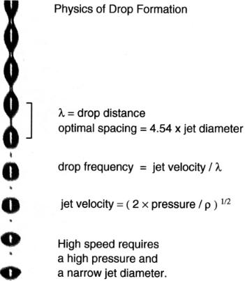
with an optimum at λ = 4.54D.

Because there is an optimal spacing of the drops, the drop rate is proportional to the jet velocity (Fig. 2.6). The velocity of a jet itself is proportional to the square root of the jet pressure (Pinkel and Stovel, 1985; Peters et al., 1985). In flow cytometry, the movement of fluid through the tubing is relatively slow, and most of the pressure energy is used in forming the rapidly accelerated jet. Ignoring resistance losses in the tubing, the work performed by the pressure system, P × ∆volume, is equal to the kinetic energy of the jet:

P · areanozzle · vjet = 1/2 mvjet2 = 1/2 areanozzle ρvjet3

Drop Generation

33

where P is the pressure, vjet is the velocity of the jet, m is the mass of the jet, and ρ is the density of the fluid. This formula leads to

vjet = 2ρP ½

Note that the jet velocity is independent of the size of the nozzle orifice. The density

of water (ρwater at 20°C is 0.998 kg/m3) is not much affected by temperature; salinity has a small effect (ρsaline,20°C = ~ 1.005 kg/m3; Denny, 1993). Saline propelled by a pressure of 1 atm (1 kgf/cm2, or 14.22 psi, 9.81 × 104 N/m2) forms a jet with a velocity of

(2 × 9.81 × 104/1.005 × 103)½ = 14 m/s

The optimal drop rate is related to pressure by

foptimal	vjet	(2P/ρ)½
	= =
	λ	4.54Djet

Note that the pressure is the pressure drop across the nozzle orifice. In cell sorters, a small but significant amount of pressure is needed to transport the fluid from the sup-

F i g . 2.6. Physics of drop formation.

34	High-Speed Cell Sorting

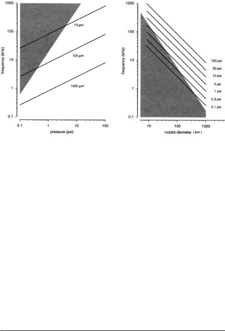
F i g . 2.7. Optimal drop generation frequencies of jets with different velocities and diameters.

ply tank to the nozzle tip. If a 70-µm nozzle receives fluid through 1 m of tubing with a 1.6-mm inside diameter (ID), the pressure drop along the tubing is ~10% of the tank pressure. In-line filters and valves cause additional losses.

These considerations lead to the nomograms of Figure 2.7, which relate pressure and drop frequency for different stream diameters and velocities. The grey zone indicates the area where the fluid drips irregularly from the nozzle because the kinetic energy is insufficient to form a jet.

These formulas and the nomogram do not take into account a number of secondary effects. The flow resistance of the walls of the nozzle orifice has been ignored. Also ignored is the contraction and acceleration of the jet as it leaves the orifice due to the redistribution of kinetic energy from a parabolic into a top-hat flow profile. At some distance from the nozzle tip, jets are somewhat (~0.85 times) narrower than the diameter of the nozzle aperture. Consequently, the velocity is not constant along the length of the jet and corrections must be applied. The nomograms are accurate to a first approximation and may serve as a guideline in generating jets and drops over a wide range of sizes and frequencies. I have found these graphs to be accurate for systems generating drops from 300 Hz at 1.5 m/s to 125 kHz at 100 psi.

FREQUENCY COUPLING

A periodic disturbance, seeded along the surface of a jet at an appropriate spacing, will rapidly grow in amplitude, eventually cleaving the jet into regular drops. A very small acoustic signal, near the optimal frequency, will be sufficient to fix the drop

Frequency Coupling

35

formation. When properly focused, the acoustic signal induces small pressure variations at the nozzle opening that cause variations in the amount of fluid exiting the nozzle aperture. Because the jet, after detachment from the nozzle tip, quickly assumes a uniform speed, the velocity variations in the nozzle orifice result in thinner and fatter regions in the jet’s girth. As discussed before, the amount of fluid leaving the nozzle varies with the square root of the pressure. The diameter of the jet in turn varies with the square root of the jet velocity. Hence, the (small) fractional variation in jet diameter is at first approximation

∆ Djet	∆ P
	= 0.25
Djet	P

Despite the small effect of pressure changes on the jet diameter, minute variations in nozzle pressure accurately determine the location of the drop boundaries. A thin piezoelement driven by 1 V or less, which corresponds to a vibration amplitude of <<100 nm, is sufficient to impose a stable drop formation onto a 70–µm jet (Fig. 2.8).

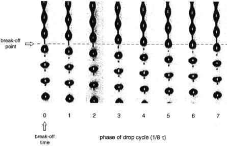
F i g . 2.8. Drop separation at the tip of the jet is a cyclical event. The figure shows eight photographs that are evenly spaced over the drop cycle. The jet moves downward with a constant velocity. The amplitude of a sinusoidal disturbance grows exponentially with time. At some point in space and time, the thin ligament that connects the last drop to the main stream snaps. The separated drop is now electrically isolated from the main stream. Moments later, the ligament separates from the drop that follows forming a microdroplet that is slightly pulled toward the tip of the jet. The microdroplet is soon overtaken by the following drop and merges with it. Note that the drop boundaries are slightly offset from the break-off point. If the stroboscopic flash that freezes the jet image is synchronous with the charge pulse, the image can be used to optimize the timing of the drop charge circuit.

36	High-Speed Cell Sorting

According to Rayleigh (1877; Kachel and Menke, 1979), the amplitude of a surface disturbance of λ > πD grows at an exponential rate with time,

a(t) = a0 eγt

and

t(a) = 1 ln a

γ a0

The growth rate γ depends on the wavelength and the overall physical characteristics of the fluid, such as viscosity and surface tension, which in turn are temperature sensitive (Denny, 1993). The time it takes for a disturbance to grow from the very small amplitude a0 at the nozzle tip to the amplitude one-half Djet that partitions the jet diameter is

γ		2a0
1		Djet
tbreak-off = ln

The variation in the break-off time as a function of the seed amplitude is

dtbreak-off	1
= –
da0	γa0
and
dtbreak-off	ln(Djet/2a0)
= –
dγ	γ2

The stability of the break-off time is inversely related to the amplitude of the seed frequency and the growth rate γ. In order to obtain a stable break-off point, the seed amplitude must be sufficiently large, and the physical properties of the fluid must remain constant. On the other hand, if the seed amplitude is too large, the disturbance will distort the optical properties of the jet, adding noise to the fluorescence and scatter measurements. Setting the amplitude of the seed frequency requires a compromise between jet stability and measurement accuracy.

NUMERICAL EXAMPLE

Experimental observations confirm the relationships described in the previous section. Figure 2.9 presents data measured with a jet generated by 30 psi from a 70-µm nozzle. Assuming a jet contraction of 0.85 and a pressure drop from tank to nozzle of 3 psi, the theoretical optimal drop frequency is ~71.5 kHz. A drop drive frequency of 71.7 kHz was found to yield the shortest jet length (distance from orifice to break-off point). The length of the jet can be expressed as time, length, or drop boundaries. The relationship between the jet length and the piezovoltage follows the theoretical predictions, indicating linearity between the drive voltage and the amplitude of the jet disturbance (Fig. 2.9). Extrapolation predicts that the jet is bisected by an amplitude corresponding to a piezovoltage of 757 V. These numbers yield a surface amplitude of ~40 nm/V. Stable