Beginning SharePoint With Excel - From Novice To Professional (2006)

96 C H A P T E R 5 ■ C R E AT I N G C U S TO M C A L C U L AT I O N S I N S H A R E P O I N T

Using the text functions LEFT and RIGHT, you can dissect the property code shown in Figure 5-3 into three distinct parts, and then easily create filtered views based on the location and property type. With SEARCH and REPLACE, you can search for text in a text string and replace it with other text.

Using REPLACE by itself, you can substitute text based on its position, including appending text to the beginning of a text string. For example, if you wanted to add

a brand name to precede names of products in a list, as shown in Figure 5-4, you could use REPLACE. The following formula inserts "FabWear " (note the space after the brand name) in the first position (1), replacing no text (0):

=REPLACE([Item],1,0,"FabWear ")

Figure 5-4. Using the REPLACE function, you can add the brand name “FabWear” to the item names.

With other text functions, such as UPPER, LOWER, and PROPER, you can convert text from one case to another; for example, “residential” to “RESIDENTIAL” or “Residential.”

Table 5-6 describes several of the most useful text and data functions.

■Tip You can concatenate fields without using the CONCATENATE function by building the formula yourself. For example, to combine [FirstName] and [LastName] into a [FullName] column displaying Last name, First name, you can create the following formula:

=[LastName]&" ,"&[FirstName]

The ampersand character joins the fields, and anything enclosed in parentheses appears as text; in this case, a space and a comma.

C H A P T E R 5 ■ C R E AT I N G C U S TO M C A L C U L AT I O N S I N S H A R E P O I N T

97

Table 5-6. Text and Data Functions Manipulate Text Strings

Function	Syntax	Description	Example	Result
CONCATENATE	CONCATENATE	Joins two or more	=CONCATENATE	Aidan Holm
	(text1,text2,...)	text strings into one.	(Holm, Aidan)
LEFT	LEFT([Column1],2)	Extracts the left two	=LEFT	Returns the first
		characters from	([PropertyCode],2)	two characters
		the string.		of the code
RIGHT	RIGHT([Column1],3)	Extracts the right	=LEFT	Returns the last
		three characters	([PropertyCode],3)	three characters of
		from the string.		the code
TRIM	TRIM([Column1]	Removes all extra	=TRIM	Changes “ baseball
		spaces from text	([" baseball cap"]	cap ” to “baseball
		except single spaces		cap”
		between words.
LEN	LEN([Column1])	Returns the number	=LEN([Item])	Returns the length
		of characters in a		of the text string
		text string.
LOWER	LOWER([Column1])	Converts characters	=LOWER[(Boston)]	“BOSTON” becomes
		to lower case.		“boston”
UPPER	UPPER([Column1])	Converts characters	=UPPER[(Boston)]	“boston” becomes
		to upper case.		“BOSTON”
PROPER	PROPER([Column1])	Converts characters	=PROPER[(Boston)]	“BOSTON” or
		to proper case		“boston” becomes
				“Boston”
SEARCH	SEARCH(find_txt,	Returns the number	=SEARCH("cap",	In string “baseball
	within_txt,	of characters where	"baseball	cap,” returns 10
	Start_num)	a character or text	cap", [10])
		string is first found.
		Find_txt is text you
		want to find;
		within_txt is the
		location (that is,
		[Column1]); Start_num
		is the number of
		characters in the
		string you want to start
		searching (optional).
REPLACE	REPLACE(old_text,	Replaces original text	=REPLACE([Item],1,	Inserts “FabWear ”
	start_num,	(old_text) with new text	0,"FabWear ")	in the first position
	num_chars,	(new_text) based on the		(1), replacing no
	new_text)	position of the first		text (0)
		character (start_num),
		and the number of
		characters (num_chars)
		you want to replace.

98 C H A P T E R 5 ■ C R E AT I N G C U S TO M C A L C U L AT I O N S I N S H A R E P O I N T

Applying Logical Functions

You use logical functions to create conditional formulas. You can use logical functions to test whether conditions are true or false, and to make logical comparisons between expressions. For example, using the IF function, you can test if the value in one column is greater or less than a specific value. If it evaluates as true, you could apply a formula to the value; if not, leave it as is.

In practical terms, let’s say you want to discount all the items in a store’s inventory that had been in stock prior to January 1. You could use the IF function to examine the DateAcquired column to determine if an item was acquired prior to January 1. If it was, you would apply the discount; if it wasn’t, you’d leave it at the current price. The formula might look like the following:

=IF([DateAcquired]>1/1/2006,[Price]-[Price]*30%,[Price])

With an IF function, the first part of the statement sets up the condition: is [DateAcquired]>1/1/2006? The second part of the statement, after the first comma, says to do this if the condition is true. In this case, you’d discount the item by 30 percent. The third part of the statement, after the second comma, says to do this is the condition is false. In this example, you’d keep the price as it is. The syntax for an IF function is as follows:

=IF(logical_test,value_if_true,value_if_false)

You can use AND, OR, and NOT functions to combine conditions and set up different conditions. For example, let’s say in the preceding example, you want to apply a 30 percent discount if the item was acquired between 10/1/2005 and 1/1/2006, and a 50 percent discount if it was older than 10/1/2006. You could do this with the AND function. The following formula contains an AND function (AND(logical1,logical2,...) that sets up the condition of dates between 10/1/2005 and 12/31/2006 (<1/1/2006) and a nested IF:

=IF(AND([DateAquired]<1/1/2006,>=10/1/2005),[Price]-[Price]*30%,

IF([DateAcquired]<10/1/2005,[Price]-[Price]*50%,[Price]))

These two IF statements are dependent on each other (for more about nested functions, see “Nesting Functions for Maximum Efficiency” later in this chapter).

Use AND when you want the condition to meet both criteria. You can use OR if you want the condition to meet either criteria; for example, if you acquired the item prior to 1/1/2006 OR the item is damaged. You could also use NOT to include only items that haven’t been damaged:

=NOT([Condition]="Damaged"

C H A P T E R 5 ■ C R E AT I N G C U S TO M C A L C U L AT I O N S I N S H A R E P O I N T

99

When creating formulas with logical functions, you can often find more than one way to develop the formula. The key is to create an accurate formula that makes sense to you. As long as it meets those criteria, it doesn’t matter which functions you choose to do it.

Table 5-7 describes the logical functions.

Table 5-7. Logical Functions Test for Conditions

Function	Syntax	Description	Example	Result
IF	IF(logical_test,	Tests to see if a condition	=IF[FlightMiles]<500,	Evaluates
	value_if_true,	is true. If it is, the formula	[FlightMiles]*50%+	whether a flight
	value_if_false)	sets the first value. If it isn’t,	[FlightMiles],	is less than 500
		it sets the second.	[FlightMiles]	miles. If it is, adds
				a 50 percent
				miles bonus.
AND	AND(logical1,	Evaluates criteria that	=AND	Evaluates to
	logical2,...)	evaluates as other than	([FlightMiles]>500,	true when
		true or false.	[FlightMiles]<1000	a flight is more
				than 500 and
				less than 1,000
				miles.
OR	OR(logical1,	Evaluates criteria that	=OR	Evaluates to
	logical2,...)	evaluates as other	([FlightMiles]>500,	true when
		than true or false.	[Destination]=	a flight is more
			"Los Angeles"	than 500 miles
				or the
				destination is
				Los Angeles.
NOT	NOT(logical)	Evaluates whether	NOT	Anywhere
		something is false.	([Destination]="Detroit")	but Detroit.

■Note TRUE and FALSE are also logical functions. However, you can type TRUE and FALSE directly into formulas without using the functions. For example, you could enter a formula that evaluated whether a statement was TRUE and if so, apply a calculation to it.

Using Information Functions

Information functions give you information about the values in a list. For example, ISBLANK looks at whether a cell in a list is blank. The information functions are particularly useful when combined with the IF function. Let’s say you want to look at clothing items in the store’s inventory and apply a different brand name depending on what the item is. If the item is a cap, you want the brand name “FabWear” to precede the item; every other item should be branded “TopWear.” By combining text, logical, and information functions, you can create a formula that accomplishes this task. It’s easiest to start with creating a column, Caps, that identifies the caps in the list. Use the SEARCH function

100 C H A P T E R 5 ■ C R E AT I N G C U S TO M C A L C U L AT I O N S I N S H A R E P O I N T

to search the [Item] column for the text “cap.” The following formula returns “cap” if it finds it, and #VALUE! if it doesn’t:

=SEARCH("cap",[Item])

You’re now ready to create the calculated Brand column using the following formula:

=IF(ISERROR([Caps]),REPLACE([Item],1,0,"TopWear "),REPLACE([Item],1,0,"FabWear "))

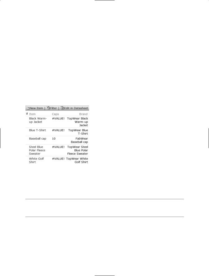
This formula starts with an IF statement that evaluates if the Caps column displays an error, using the ISERROR function (this error is represented by #VALUE!). If it does, the formula uses the REPLACE function to insert “TopWear” at the first position in the string. If it doesn’t, it inserts “FabWear” into the first position of the string. Figure 5-5 shows the results of this formula.

Figure 5-5. In this list, the Caps columns identifies the items that contain the text string “cap,” and the Brand column shows the results of applying the appropriate brand names to the items.

■Tip If you create a column solely for the purpose of calculations, create a custom view that doesn’t display the column. See Chapter 4 for more about creating views.

Table 5-8 details the most common information functions.

C H A P T E R 5 ■ C R E AT I N G C U S TO M C A L C U L AT I O N S I N S H A R E P O I N T

101

Table 5-8. Information Functions Give You Information About Values

Function	Syntax	Description	Example	Result
ISBLANK	ISBLANK(value)	Identifies an empty cell.	=ISBLANK	Evaluates as true if the
			([MiddleName])	MiddleName column
				is empty.
ISERR	ISERR(value)	Refers to any error	=ISERR	Evaluates as true if the
		value except #N/A.	([MiddleName])	cell contains any value
				except #N/A.
ISERROR	ISERROR(value)	Refers to any error	=ISERROR([CAPS])	Evaluates as true if an
		value (#N/A, #VALUE!,		error value displays in
		#REF!, #DIV/0!, #NUM!,		the cell.
		#NAME?, or #NULL!).
ISNA	ISNA(value)	Refers to the #N/A	=ISNA	Evaluates as true if the
		(value not available)	([MiddleName])	cell contains #N/A.
		error value.
ISNONTEXT	ISNONTEXT(value)	Refers to any item that	=ISNONTEXT	Evaluates as true
		isn’t text. (This function	([FlightMiles]	if the cell is blank
		returns TRUE if the		or contains a value
		value refers to a blank cell.)		that is not text.
ISNUMBER	ISNUMBER(value)	Refers to a number.	=ISNUMBER	Evaluates as true if the
			([FlightMiles])	cell contains a number.
ISTEXT	ISTEXT(value)	Refers to text.	=ISTEXT	Evaluates as true if the
			([FlightMiles])	cell contains text.

Nesting Functions for Maximum Efficiency

Although it’s possible to create multiple columns to create formulas that are based on the results of a function, you can also nest functions into one formula. SharePoint supports up to eight levels of nested functions. To nest a function, you include a secondary function inside the primary function. For example, if you want to sum three columns and then round the result, you’d create a formula similar to the following:

=ROUND(SUM[Column1],[Column2],[Column3]))

Using the order of operations, this sums the three columns and then applies the ROUND function to the result.

SharePoint isn’t very helpful in suggesting where an error exists in a formula. When creating formulas with nested functions, you might want to create them in stages, testing each part of the formula as you go along. In the example in the previous paragraph, you could create the SUM function and review the results in the column. If it’s correct, you could then add the ROUND function to the formula. In this way, you can narrow down the possible errors as you go along.

102 C H A P T E R 5 ■ C R E AT I N G C U S TO M C A L C U L AT I O N S I N S H A R E P O I N T

■Note The most common error when creating nesting formulas is omitting the closing parentheses at the end of each function. Excel automatically prompts you to fix this error; SharePoint does not. You have to figure out the error for yourself.

Summary

Formulas add extra functionality to a SharePoint list. The list is no longer a static data repository, but an active part of your collaboration work with your team. Much of the same functionality you have in Excel is available in SharePoint lists. You can apply formulas using references, operators, constants, and functions. SharePoint offers 150 functions, from simple math functions such as SUM to complex statistical functions such as DEVSQ (returns the sum of squares of deviations of data points from their sample mean). In this chapter, we identified many of the most commonly used and most helpful functions.

In a SharePoint list, you can add column totals to a list, but you cannot create formulas based on these totals. Formulas can be based only on data within a row, not on column data. To combine multiple functions into one formula, you can create nested functions.

SharePoint isn’t helpful in identifying the possible source of an error in a formula, so by constructing the formula in steps, you can test each part of the formula as you go along.

In Chapter 6, we’ll look at options for publishing Excel workbooks as web pages to a SharePoint site.

C H A P T E R 6

■ ■ ■

Publishing Excel Web Pages for SharePoint

In previous chapters, we’ve shown you how to take advantage of the built-in integration between SharePoint lists and Excel lists. If all the data stored in Excel workbooks was stored in lists, this book would have only five chapters. But Excel is so much more—and so is SharePoint. SharePoint is a great platform for Excel reports, whether the data you want to share is a chart, a table, or an entire workbook. In this chapter, we’ll show you how to publish Excel information as HTML, and then use this file in on your SharePoint site. Using Excel’s web tools, you can publish workbooks, worksheets, charts, and pivot tables.

When you save or publish Excel worksheets as web pages, the pages you create are either static or interactive. Static pages are simple stationary pages you could publish in every version of Excel since Excel 97. Interactive pages include the Office Web Components, which empower users by letting them work directly with Excel data in their browser using Excel tools, turning the web page into a decent ad hoc report and analysis tool. Interactive web pages let users add formulas, sort and filter data, analyze data, and edit charts.

Creating a Web Page in Excel

Not every report user is an Excel user. A workbook saved as a web page is friendlier and more accessible for users than an Excel workbook, and practically foolproof. All users can view the web page, even if they’re viewing it on a Mac, or on a PC that doesn’t have Excel installed.

Saving an entire workbook as a static web page is an easy process: open the workbook, check the workbook’s formatting, set the page title, then save it as a web page.

103

104 C H A P T E R 6 ■ P U B L I S H I N G E X C E L W E B PA G E S F O R S H A R E P O I N T

Formatting the Workbook Before Saving

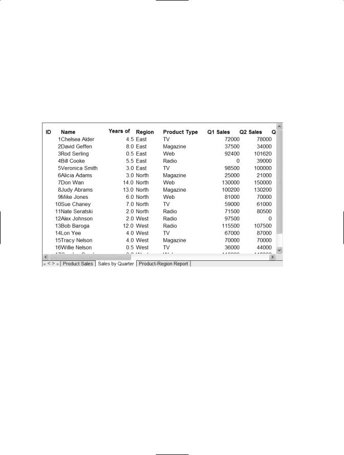
Review the workbook’s the column widths, alignment, and other formatting, and adjust formatting if appropriate. You can’t easily modify formatting in the saved web page. In the file shown in Figure 6-1, there’s no space between the ID numbers in column 1 and the names in column 2. The column heading in the third column, Years of Service, is truncated. These are examples of issues that are most easily corrected in Excel prior to saving the web page.

Figure 6-1. Adjust column widths, text wrapping, and numeric formatting before saving the workbook as a web page.

In Excel, apply a numeric format (not General) to all numbers, even a column of simple integers, such as those in the first column of Figure 6-1. Edit long column headings to make them shorter, and align column headings to reflect the alignment of the data in the column. To see the difference a few simple formatting changes can make in the published web page, see Figure 6-4 later in this chapter.

If your workbook includes workbook or worksheet protection, you must remove it before saving the workbook as a web page. Otherwise, it can’t be saved (a warning message appears when you try to save a protected workbook as a web page).

Saving the Workbook As a Web Page

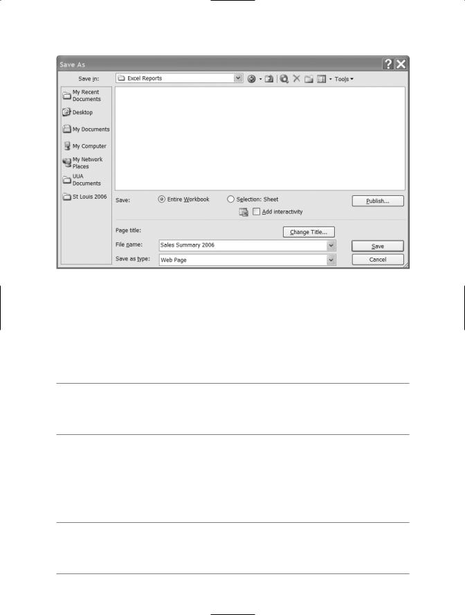
To save the entire workbook as a web page, select any single cell in the workbook. Do not select a range of cells. Choose File Save as Web Page to open the Save As dialog box, shown in Figure 6-2.

C H A P T E R 6 ■ P U B L I S H I N G E X C E L W E B PA G E S F O R S H A R E P O I N T

105

Figure 6-2. Use the Save As dialog box to create a static or interactive web page to display Excel data.

Make sure you select the Save Entire Workbook option. The default file name for the web page is the workbook name with an HTM extension. It’s good practice to edit the file name to remove spaces.

■Note In a URL, each space is replaced with %20, so each space adds three characters to the length of the URL. URLs are limited to 255 characters. If there are spaces in site names, folder names, and library names, you can easily exceed this limit when you save the HTML file on your SharePoint site.

Choose your file location with care. When you create the web page, Excel will create a main file and a folder with supporting files. SharePoint’s file upload doesn’t support uploading folders, so moving the file and folder to SharePoint later isn’t impossible, but it’s a bit complex. It’s best if you save the web page on your SharePoint site.

■Tip We create a document library named “webpages” in every Windows SharePoint Services site. All web pages displayed on the site, including pages created in Excel, are saved in the webpages document library. The webpages library isn’t listed on the Quick Launch bar.