Beginning SharePoint With Excel - From Novice To Professional (2006)

A P P E N D I X A

■ ■ ■

Creating and Using Excel Lists

Throughout this book, we’ve referred to Excel lists, the feature of Excel that makes it possible to synchronize worksheet data with SharePoint (see Chapter 2). Whether or not you want to synchronize a list with SharePoint, using Excel’s List command can simplify data entry and put features such as filter, sort, and totals at your fingertips.

Although theoretically any Excel worksheet with columns and rows of data can be called a list, Excel’s List command segregates a defined range of cells from the rest of the worksheet, making it possible to combine multiple lists into a single worksheet. Additionally, an Excel list automatically copies formulas and formatting to new rows of data, eliminating the need to do this manually. In this appendix, we’ll demonstrate the advantages of using Excel’s List command over maintaining lists the traditional way.

Creating a New List

Creating a new list is as simple as entering data into a blank worksheet. A header row isn’t required, but comes in handy for other things you might want to do, such as filtering the list. The best way to start is to enter column headings into the worksheet. Follow these steps to create the list:

1.Open a blank worksheet or select an existing worksheet that’s large enough to accommodate the list.

2.Enter column headings.

3.Select the column headings.

4.Select Data List Create List, or right-click the selected headings and click Create List from the context menu.

217

218A P P E N D I X A ■ C R E AT I N G A N D U S I N G E X C E L L I S T S

5.In the Create List dialog box, verify that the correct range is defined in the “Where is the data for your list?” text box. If it isn’t, click the Collapse button at the right end of the text box and reselect the data.

6.Select the My list has headers checkbox.

7.Click OK to create the list.

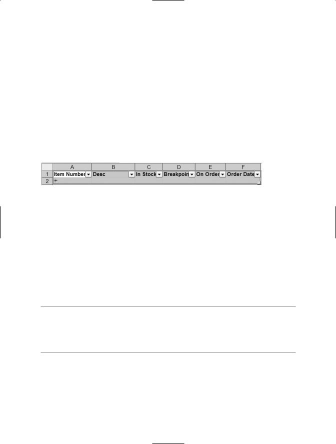
Excel automatically activates the List toolbar and draws a border around the list, separating it from the rest of the worksheet. In addition, it adds a new record row, designated by an asterisk, and turns on AutoFilter, as shown in Figure A-1. When you click outside the list, the List toolbar turns off, the AutoFilter buttons are no longer visible, and the border changes to a thin blue line. Click back inside the list to reactivate the list features.

Figure A-1. The Excel list has the AutoFilter turned on and a new row for data entry.

Entering Data into a List

To add data to the list, click in the new record row—the row with an asterisk—and start typing. When you reach the end of the row, press Enter to enter the next record.

If you want to add formulas to the list, enter the formula in the first row of data. Excel automatically copies the formula to new rows.

You can also apply text and number formatting to individual cells, and apply conditional formatting to cells or to the entire row. Excel copies the formatting to new rows you enter, and applies conditional formatting as appropriate.

■Note If you apply formula-based conditional formatting to the first row, be sure to create the formula to use a relative row reference. For example, in the Conditional Formatting dialog box, change the formula =$B$2="LGA" to =$B2="LGA" to make the column reference B absolute but the row reference 2 relative. This assures that Excel formats the data based on the current row, rather than referring only to the first row of data.

When you’ve finished entering data, click outside the list to deactivate it.

■Note

A P P E N D I X A ■ C R E AT I N G A N D U S I N G E X C E L L I S T S

219

Redefining the Columns in a List

By default, when you type a header for a column that’s adjacent to a defined list, Excel automatically expands the list to include it. List AutoExpansion is one of Excel’s AutoCorrect options. If you didn’t intend for the column to be added to the list, you can click the AutoCorrect Options button that appears next to the column and click Undo List AutoExpansion. To turn off this option permanently, click Stop Automatically Expanding Lists. You can also insert a column in the middle of a list, and Excel expands the list range to include it.

If the AutoCorrect Options button doesn’t appear, you might have AutoCorrect turned off. To activate it, select Tools AutoCorrect Options and click the Show AutoCorrect Options buttons checkbox on the AutoCorrect tab of the AutoCorrect dialog box.

If you want to change the range of columns and rows included in a list, click List on the List toolbar, then click Resize List. You can enter or select a new list range, with a couple caveats: you cannot change the header row of the existing list, and the new list range has to overlap the existing list range. In other words, you can’t change a list that was A1:D57 and make the new list E1:G57.

Deleting List Data

You can delete columns and rows in a list without affecting other data in the worksheet. Select the cells in the row you want to delete, rather than selecting the entire row. Then select Edit Delete Row, or right-click the selected cells and click Delete Row from the context menu. This deletes a row in the list without impacting data in the worksheet row that’s outside the list. For example, say you have a list range of A1:K47. You have another list range of M1:S75. By selecting just the cells you want to delete, you can delete the data in A13:K13 without deleting the data in M13:S13.

Using Database Features and Functions

One of the advantages of using Excel’s List command is the ease with which you can sort and filter lists, and toggle totals on and off.

220 A P P E N D I X A ■ C R E AT I N G A N D U S I N G E X C E L L I S T S

Sorting and Filtering

When you create a list, Excel automatically turns on AutoFilter. The AutoFilter buttons appear on the header row of the list. To sort data in the list, click the down arrow on the column you want to sort. Scroll to the top of the list, then click Sort Ascending or Sort Descending.

To filter data, select the criteria on which you want to filter from the list of values. If you want to create a custom filter, follow these steps:

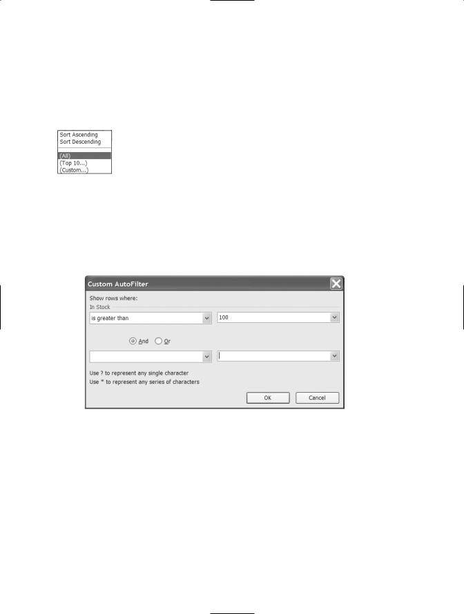
1.At the top of the drop-down list, choose (Custom) to open the Custom AutoFilter dialog box, shown in Figure A-2. Enter up to two custom filter criteria separated by AND or OR.

Figure A-2. Create a custom filter to display records that meet one or two criteria.

2.Choose from the list of comparison terms such as equals, does not equal, is greater than, and is less than, then enter or select the value. This creates the filter statement, such as the following:

Show rows where State/Prov equals Alaska or Show rows where Revenue is greater than or equal to $50,000.

3.Click OK to apply the filter. Excel hides any rows in the list that don’t meet the filter criteria.

A P P E N D I X A ■ C R E AT I N G A N D U S I N G E X C E L L I S T S

221

You can apply multiple filters to a list by filtering on more than one column. For example, if you want to see all the rows where Revenue is greater than or equal to $50,000 and State/Prov equals Alaska, you’d apply a filter to both the Revenue column and the State column.

■Tip To decide whether to use AND or OR in a custom filter, ask yourself this question: in a single row of data, do I want to see the row only if it meets both criteria (AND), or do I want to see the row if it meets either criteria (OR)?

If the AutoFilter buttons distract you, you can turn them off. Select Data Filter AutoFilter to toggle off the buttons. Repeat the same steps to turn them back on again.

Adding Totals

The Toggle Totals Row button on the List toolbar lets you toggle totals on and off at your discretion. Totals aren’t limited to sums—the Totals row includes the choice of eight functions: Average, Count, Count Nums, Max, Min, Sum, StdDev, and Variance. To display totals, follow these steps:

1.Click the Toggle Totals Row button on the List toolbar.

2.In the row labeled Totals, click the cell that’s in the column you want to total.

3.Select the totals function you want to apply from the drop-down list. Excel displays the applicable total in the cell.

4.Move to the next column you want to total and repeat step 3.

When Excel adds a totals formula in the Totals row to a list, it doesn’t just create a standard formula, such as =SUM(D3:D59). Instead, it inserts a subtotals formula, such as =SUBTOTAL(109, D3:D59), where the first argument (in this case, 109) represents the SUM function. The SUBTOTAL function ignores hidden values. The advantage of SUBTOTAL over SUM, AVERAGE, and the other aggregate functions is that it doesn’t matter if the data is filtered or not. A correct total is always displayed.

■Note The syntax for the SUBTOTAL function is as follows:

(SUBTOTAL(function_num, ref1, ref2, ...)

222 A P P E N D I X A ■ C R E AT I N G A N D U S I N G E X C E L L I S T S

Table A-1 shows the function numbers (function_num) for each of the available aggregates used in the SUBTOTAL function.

Table A-1. Subtotal Function Numbers

Function	Function_num
AVERAGE	101
COUNT NUMS	102
COUNT	103
MAX	104
MIN	105
STDDEV	107
SUM	109
VARIANCE	110

■Note In case you’re wondering, the missing function numbers (function_num) are PRODUCT (106), which multiplies all the arguments; STDEVP (108), the standard deviation of a population; and VARP (111), the variance of a population. If you use function numbers 1–11, the SUBTOTAL function includes hidden values; function numbers 101–111 hide hidden values.

When you’re adding records to the list, you might find it easier to toggle the Totals row off. To do that, just click the Toggle Totals Row button on the List toolbar again.

When Lists Don’t Work

Excel’s List command is great to use for a lot of your list needs. However, you cannot use Excel lists with the following items:

•Shared workbooks: You must unshare the workbook before you can convert a range to a list, or convert the list to a normal range to share a workbook that contains

a list.

•Compare and merge workbooks: You must convert the list to a normal range before you can compare and merge workbooks.

A P P E N D I X A ■ C R E AT I N G A N D U S I N G E X C E L L I S T S

223

•Subtotals: Excel lists automatically display subtotals using the Totals row (the Toggle Totals Row button on the list toolbar). However, you cannot have Excel automatically insert subtotal rows after categories of data. If you need a subtotals report, convert the list to a normal range.

•Custom views: You must convert the list to a normal range to create custom views of the worksheet, as covered in the following section.

Converting a List to a Normal Range

If you need to use a feature that Excel’s List command doesn’t support, you can temporarily or permanently convert the list to a range. To convert a list to a range, right-click the list, then select List Convert to Range. Alternately, click List on the List toolbar and click Convert to Range. Confirm your choice by clicking Yes when prompted: “Do you want to convert your list to a normal range?” Excel removes the border around the list, deactivates the List toolbar, and turns off the AutoFilter buttons.

To convert the data back to a list, follow the directions in the section “Creating a New List” earlier in this appendix. The only difference is that you want to select the entire range of cells that contain data.

A P P E N D I X B

■ ■ ■

Mapping Excel Spreadsheets for XML

In 1998, the World Wide Web Consortium (W3C) posted goals for a new language that would facilitate data transfer between computers and systems. According to the goals, the new Extensible Markup Language, or XML, would meet specific criteria. The XML draft document describes a standard language with optional features “kept to an absolute minimum,” resulting in easy-to-create, human-readable documents. In less than a decade, XML has moved from a set of goals to a language that has undergone frequent and rapid revision. Excel 2003 includes native support for XML (as does Access and InfoPath). In the next version of Office, 2007 Microsoft Office System, every Office application will include native XML support. If you work with SharePoint and Excel, you can’t ignore XML.

XML Basics

XML describes data as a hierarchy: a company has departments, departments have employees, employees have first names and last names, and so on. The following simple XML file describes one “record”—an e-mail message:

<?xml version = "1.0" ?>

<MESSAGE>

<TO>[e-mail]</TO>

<CC>[e-mail]</CC>

<FROM>[e-mail]</FROM>

<DATE>06/01/06</DATE>

<SUBJECT>New Office Location</SUBJECT>

<BODY>Where should this item appear on the meeting agenda?</BODY>

</MESSAGE>

225