Beginning SharePoint With Excel - From Novice To Professional (2006)

46 C H A P T E R 3 ■ W O R K I N G W I T H S H A R E P O I N T L I S T S I N E X C E L

Working with Offline Data in Excel

Working with the SharePoint data in Excel is similar to working with an Excel list that’s been previously published in SharePoint. You don’t have to be online to edit the SharePoint list data, even while online users are working with the SharePoint list. You can edit the list and add rows (records), then save the workbook locally until you’re back on the network and ready to synchronize your offline data with the SharePoint list.

If you have a group of users who need to update the same data set, a SharePoint list allows each user to export and work with the data independently and simultaneously. As you’ll see, SharePoint manages any conflicts that occur when two or more users make different changes to the same data element.

Many users prefer to work with their SharePoint lists offline in Excel:

•Managers: During budget “crunch time” when they’re finalizing line items and many users need to update different rows in the same list

•Sales people: Logging sales leads and customer information on the road instead of waiting until they return to the office

•Developers: Recording actions taken to resolve items in an Issues log

•Information workers: Editing lists during peak hours on a slow network

•Frequent flyers and other travelers: Working with list data when they don’t have access to their corporate SharePoint site

SharePoint Calculated Fields in Excel

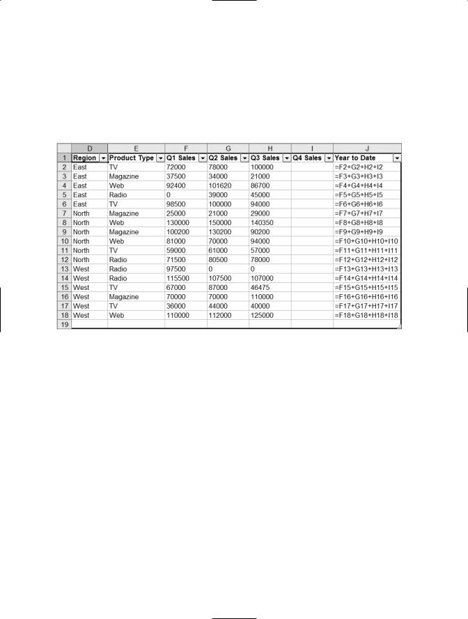
If the SharePoint list you exported to Excel includes calculated fields, the calculations are reflected in the Excel list. For example, the Sales by Quarter SharePoint list shown in Figure 3-7 includes a calculated Year to Date column.

Figure 3-7. Portion of a SharePoint list with a calculated field,Year to Date

C H A P T E R 3 ■ W O R K I N G W I T H S H A R E P O I N T L I S T S I N E X C E L

47

The following calculation is used for the Year to Date field:

=[Q1 Sales]+[Q2 Sales]+[Q3 Sales]+[Q4 Sales]

When the list is exported to Excel, Excel converts the SharePoint formula to an Excel formula, as shown in Figure 3-8.

Figure 3-8. Calculated fields in SharePoint are converted to formulas in Excel.

The formulas are automatically protected in Excel. Users aren’t allowed to overwrite or edit the calculated fields from SharePoint (for more about calculations in SharePoint, see Chapter 5).

Adding Calculations in Excel

You can add more columns of data in Excel and use the SharePoint list data in your calculations. Add fields starting with the first column to the right of the query results. To have Excel automatically fill the formulas down if the query data returns additional rows, modify the external data source properties:

1.On the List toolbar, click the List button.

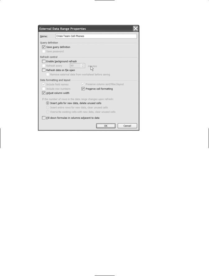
2.Choose Data Range Properties from the menu to open the External Data Range Properties dialog box (see Figure 3-9).

48 C H A P T E R 3 ■ W O R K I N G W I T H S H A R E P O I N T L I S T S I N E X C E L

Figure 3-9. Enable the “Fill down formulas” checkbox to copy formulas automatically.

3. Select the Fill down formulas in columns adjacent to data checkbox. Click OK.

When you refresh the query data, Excel will automatically fill formulas in columns to the right of, and adjacent to, the query results if the query returns additional rows.

Synchronizing the Offline Data with SharePoint

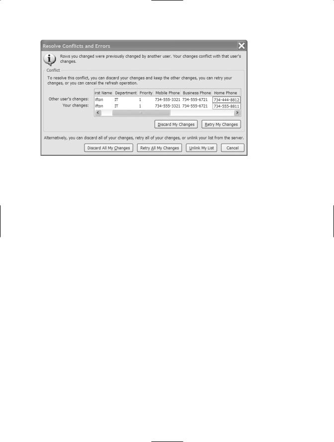
When you’re ready to synchronize your offline data, save the file locally and then click the Synchronize button on the List toolbar. If your synchronization causes a conflict because it includes changes to a data element that another user has already changed, the Resolve Conflicts and Errors dialog box opens, shown in Figure 3-10 (see Chapter 2 for more information about synchronization).

C H A P T E R 3 ■ W O R K I N G W I T H S H A R E P O I N T L I S T S I N E X C E L

49

Figure 3-10. Resolve conflicts that occur when more than one user changes the same data.

Finally, you can choose to unlink your offline Excel list from the SharePoint list. You can’t undo this choice, and if you unlink the list, you won’t be able to synchronize the list with SharePoint in the future. If you want to retain the changes you made in Excel without handling any conflicts—perhaps so you can examine the list in SharePoint—click Cancel rather than unlinking the list.

Note that the first user is never asked to deal with a data conflict. It’s the second user’s changes that create the conflict. If a number of people are working with offline copies of the same SharePoint list and editing the same rows, it’s a good strategy to synchronize frequently. The longer you wait to synchronize, the greater the possibility that another user has already synchronized a change to a list element you also edited.

If you’re at the end of a project or process and won’t be using the offline Excel data for a while, you can delete the worksheet or workbook. It’s easy enough to create another, fresh offline Excel data set when you need to work with it in the future. If you’ve added other calculations in Excel, though, you might not want to discard the worksheet or workbook casually. The next time you open the workbook, begin by synchronizing so you start with the current data from SharePoint. If you begin with old data, you increase the potential for conflicts when you synchronize.

Scenario: The Crisis Response Team System

Most organizations have a crisis or disaster response team: a group of people from various departments who are immediately contacted in case of an emergency. When the power goes out in Michigan and New York, the levees break in New Orleans, or the wind and rain come ashore in Florida, someone pulls out the crisis response plan and starts making phone calls. This is an application that you can create easily using a SharePoint list and offline Excel lists.

50 C H A P T E R 3 ■ W O R K I N G W I T H S H A R E P O I N T L I S T S I N E X C E L

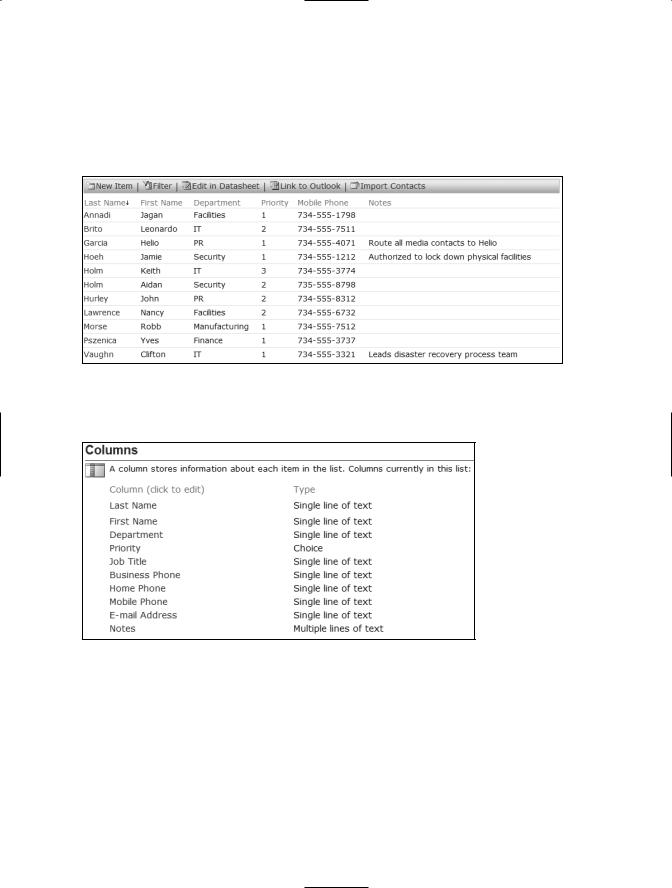
We started with a SharePoint Contacts list customized by adding columns for Priority (a choice list indicating who is called first, second, and third) and Department, shown in Figure 3-11. The specifications for the columns from the Crisis Response Team SharePoint list are shown in Figure 3-12.

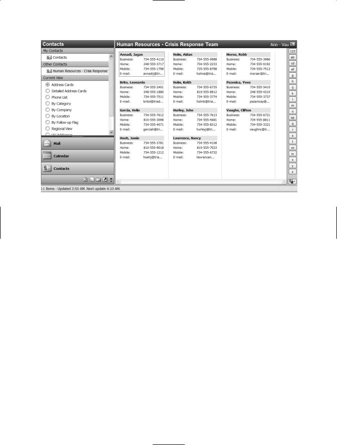
Figure 3-11. The Crisis Response Team list includes contact information for all members of the team.

Figure 3-12. SharePoint column list for the Crisis Response Team list

Team members and employees in the organization’s security department must have fast and direct access to this list. It’s a SharePoint contacts list, so this is easy to accomplish. Anyone who wants access to the list can click the Link to Outlook button to add the Crisis Response Team list to Outlook, as shown in Figure 3-13.

C H A P T E R 3 ■ W O R K I N G W I T H S H A R E P O I N T L I S T S I N E X C E L

51

Figure 3-13. Team members can add the Crisis Response Team to Outlook with just one click.

Outlook automatically keeps this list synchronized with the list on the SharePoint site, and Outlook provides a number of different page setups (card style, booklet, phone list) that the team members can use to print the team’s contact information to keep at home or in their car. They need a hard copy of the list when the power goes out!

Every month, each department manager is required to update the information for his or her department. Department managers can export the list to Excel and make their changes offline, then synchronize their changes. A SharePoint list exported to Excel, changes in Excel synchronized to SharePoint, SharePoint synchronized to Outlook on team members’ desktops: a powerful system created using the built-in functionality of Excel, SharePoint, and Outlook.

Charting SharePoint Data in Excel

Windows SharePoint Services and SharePoint Portal Server include specialized web parts to create charts and pivot tables for use on SharePoint sites. But you don’t have to do all your charting on a web site. After you’ve exported SharePoint data to Excel, you can do anything with it that you can do with native Excel data, including creating charts to illustrate the data.

52 C H A P T E R 3 ■ W O R K I N G W I T H S H A R E P O I N T L I S T S I N E X C E L

■Note Placement is important. If a query returns ten rows this time, it might return eight or fifteen next time, so you shouldn’t place charts below the query results. Locate charts above or to the right of the query results, or on another worksheet.

In Excel, select the exported SharePoint data you wish to chart, then click the Chart Wizard button on the Standard toolbar to launch the Chart Wizard. Create the chart as you would with native Excel data.

You don’t need to export the data first. You can launch Excel’s Chart Wizard directly from SharePoint. Follow these steps to create a chart directly from SharePoint:

1.Open the list you want to chart in Datasheet view. If it’s in Standard view, click the Edit in Datasheet button on the list toolbar to switch to Datasheet view.

2.Click the Task Pane button to open the task pane.

3.Click the Chart with Excel link to open Excel, return the query results, and launch the Chart Wizard with all the query results selected.

4.Complete the steps of the Chart Wizard to create the chart.

■Note If you have a SharePoint list that’s often used for a chart, consider creating a view, Chart Data, that only includes the columns needed for the chart. For information on creating views, see Chapter 4.

Creating PivotTable and PivotChart Reports

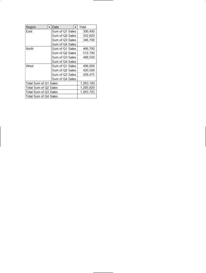
PivotTable reports are tables that organize and summarize information for easier analysis. PivotChart reports are graphical representations of the same data. PivotTable and PivotChart reports are interactive; you can move information around to compare data and look for trends and relationships. A PivotTable report of the Sales by Quarter data shown earlier in this chapter is displayed in Figure 3-14.

C H A P T E R 3 ■ W O R K I N G W I T H S H A R E P O I N T L I S T S I N E X C E L

53

Figure 3-14. A PivotTable report of the Sales by Quarter data

There are four areas in a PivotTable report: Data, Rows, Columns, and Page. Numerical data is summarized in the Data Area. Columns that describe the data are placed in the Rows and Columns Areas. Columns used to group data are placed in the Page Area. In the PivotTable report shown in Figure 3-14, the Region field was dropped in the Row Area. The four fields containing sales data (Q1 Sales, Q2 Sales, Q3 Sales, and Q4 Sales) were placed in the Data Area.

As with charts, you can create PivotTables and PivotCharts directly from a SharePoint datasheet view, or create reports with SharePoint data previously exported to Excel. There’s a difference between the two methods. When you create PivotTables and PivotCharts using the SharePoint Datasheet view task pane, the query doesn’t export the data from the SharePoint list to the Excel workbook. The report is linked directly to the data in the SharePoint list (to create and display PivotTables and PivotCharts on a page in a SharePoint site, see Chapter 9).

Creating a PivotTable Report from SharePoint

To create a PivotTable report directly from SharePoint, follow these steps:

1.Display the list in a datasheet view.

2.Click the Task Pane button to display the task pane.

3.Click the Create Excel PivotTable Report link in the task pane to launch Excel.

4.When the Opening Query dialog box opens, click Open to run the query.

54C H A P T E R 3 ■ W O R K I N G W I T H S H A R E P O I N T L I S T S I N E X C E L

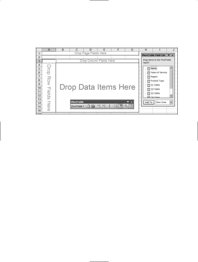
5.In the Import Data dialog box, choose a location for the PivotTable report. The PivotTable, PivotTable Field List, and PivotTable toolbar are automatically displayed, as shown in Figure 3-15.

Figure 3-15. To create a PivotTable, drag fields from the list and drop them in the four areas of the PivotTable.

6.To create the PivotTable, drag fields from the Field List and drop them in the areas of the PivotTable.

Changing Field Settings

When you drop a field that contains numbers in the Data Area, Excel uses the Sum function to summarize the data in the field. If you drop a field that contains any non-numeric data, Excel uses the Count function to summarize the data. The field names used to describe the fields start with the summarization method (Sum of, Count of), followed by the field name.

To change the summarization method or the field name, right-click the field name and choose Field Settings from the context menu to open the PivotTable Field dialog box, shown in Figure 3-16.

C H A P T E R 3 ■ W O R K I N G W I T H S H A R E P O I N T L I S T S I N E X C E L

55

Figure 3-16. Change the summarization method and other field settings in the PivotTable Field dialog box.

To change the summarization method, choose another method from the “Summarize by” drop-down list.

To change the field name, enter a new name in the text box. You cannot use the name of a source field. For example, in Figure 3-16, you cannot name the field Q1 Sales, but you can rename it Sales - Q1.

Pivoting the PivotTable Report

Interactivity is what puts the “pivot” in PivotTable reports. You can rearrange the report by moving fields between the Row, Column, and Page areas. Figure 3-17 shows the PivotTable report from Figure 3-14 after the Region field has been dragged from the Row Area to the Column Area.

Figure 3-17. Drag fields from one area to another to modify the PivotTable report.