Tools Menu

Measurement Dialog

TracePro provides a tool to display information for different entity types in the Model along with the relationship between two entities. The entities that can be used are Surface, Edge and Vertex. The dialog, shown in Figure 6.48, provides a selection of the Measurement Type based on the combination of entities to be measured. The combinations may be:

•Vertex - Vertex

•Vertex - Edge

•Vertex - Surface

•Edge - Edge

•Edge - Surface

•Surface - Surface

FIGURE 6.48 - Measurement Dialog showing edge information and distance between two selected edges

After the Measurement type is selected, TracePro will prompt for two selections. After each selection information pertinent to the entity type is displayed. The relationship between the two entities is displayed after the second item is selected. The relationship is the closest distance between the two entities, the transverse or delta distances between the entities, and the positions upon the two entities from which the distances are calculated. The information is displayed in Model Units and angles are displayed in degrees.

The Cursor will change to indicate the type of selection required.:

•	Vertex Selection Cursor
•	Edge Selection Cursor
•	Surface Selection Cursor

TracePro 5.0 User’s Manual

6.63

Analysis

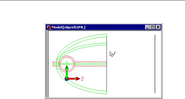
Figure 6.49 shows a model with an Edge-Edge measurement after the two edges have been selected. The Cursor shows that an edge can be selected to continue the next measurement.

FIGURE 6.49 - Elliptical Reflector with two edges selected for measurement

Figure 6.48shows the result of the measurement. When an edge is selected its starting and ending positions are displayed in Model Units. The position is displayed for a vertex. The distance is given as the minimum distance between the two selections.

6.64	TracePro 5.0 User’s Manual

CHAPTER 7	Technical Reference

Introduction

This chapter contains detailed information for many aspects of TracePro. Similar topics appear in prior chapters giving general details and have referenced this chapter for in depth coverage. Generally you can refer to the topics in this chapter as needed.

The Use of Ray Splitting in Monte Carlo Simulation

Monte Carlo simulation is a field unto itself and is used to simulate many different types of physical processes. Whenever processes are treated stochastically, with samples chosen randomly and probability distributions used to model physical processes, it is called Monte Carlo. In optics, the rays are the samples and specular reflection and transmission, reflective and transmissive scattering, and absorption are the processes. The Monte Carlo technique originates in the Manhattan project during World War II, where it was used to simulate neutron transport in fissionable material. The first computer on which Monte Carlo simulations were done was a room full of people with calculators at Los Alamos, supervised by the scientists there. Later at Los Alamos, the first electronic computer was used to do Monte Carlo simulation. After the war and into the 1950s, Monte Carlo techniques were enhanced with variance reduction techniques to vastly improve the speed of convergence of Monte Carlo simulations. The most successful of these are splitting, importance sampling, and stratified sampling. These techniques are still in widespread use today.

In the late 1950s and early 1960s, Monte Carlo was first used to trace rays, not for optical simulations, but for simulation of radiative heat transfer. On those early computers with limited processing power, they implemented what was called “crude Monte Carlo” or Monte Carlo without any variance reduction. In the late 1960s, the first optical Monte Carlo program was developed: GUERAP. It used both splitting and importance sampling for variance reduction. TracePro embodies the same variance reduction techniques as GUERAP.

Also in the late 1960s, the first workers in computer graphics were making pictures on line printers using crude Monte Carlo, which they dubbed “photon tracing.” In crude Monte Carlo, a ray would retain all of its flux, and be either fully absorbed or fully transmitted. Crude Monte Carlo does in fact conserve energy, but also suffers from slow convergence, i.e. large variance for a given sample population.

Ray Splitting as applied to ray tracing means that rays are split into different components, each carrying a fraction of the incident flux. For each ray incident on a surface, with Ray Splitting ON and 1 Random Ray per scatter selected, TracePro creates up to four rays (specular R and T, scattered R and T) leaving the surface. The sum of the flux of the four rays is equal to the flux of the incident ray less any absorption at the surface (absorption can be considered as a fifth split ray that doesn't propagate).

The truth of the matter is that, except in rare cases, the use of variance reduction (including ray splitting) does reduce the variance, and sometimes in very dramatic