Analysis

5.Change the ray color by clicking in the Color cell and selecting the new color from the Color Picking dialog

6.Press the Replace Custom Palette button

7.Press Update Ray Colors

Note: the Custom Color Palette will be stored in the OML file.

Wavelength-based ray colors

This section of the Ray Colors dialog box allows you to display the rays in either of:

•Red to Blue (false color)

•Color of wavelength (non-visible wavelengths in black)

With Red to Blue (false color) coding, rays will be colored in descending order of to wavelength from red to blue (long to short wavelengths). With Color of wavelength coloring, the color of each wavelength, according the CIE 1936 standard, will be used to display the rays for that wavelength.

Source-based ray colors

This section uses the color of each source to color the rays. The source color can be changed by clicking on the color bar and selecting a new color. The color can also be changed in the source definition.

All rays one color

You can choose to have all rays displayed in the same color. The default color is black. You can change the color by clicking on the color bar.

Irradiance Maps

Irradiance or illuminance maps can be viewed by selecting Analysis|Irradiance Maps. An irradiance map will be displayed showing irradiance incident on the currently selected surface. If the surface is not a plane, the irradiance will be projected onto a plane. The orientation of the projection plane is controlled in the irradiance Options dialog box accessed from Analysis|Irradiance Options...,or by right clicking in the Irradiance Map window and selecting Irradiance/Illuminance Options... Other settings, as described below, are controlled within this dialog. The map can be displayed in shades of gray with white being the highest irradiance and black being zero irradiance, vice versa, or in one of a selection of false color palettes.

The orientation of the irradiance map is determined by the Normal Vector and the Up Vector, as specified in the Analysis|Irradiance Options dialog box. The normal vector is normal to the projection plane on which the map will be displayed, and the up vector determines which side of the map will be at the top of your screen. The normal vector can be defined to point out from or into an object. Reversing the direction will cause the image to be flipped from left to right. If, upon displaying the irradiance map, it seems nonsensical, check the orientation of these vectors. You can have TracePro choose the Normal and Up vectors by clicking Automatically calculate Normal and Up Vectors. Click Apply to update the display.

6.4	TracePro 5.0 User’s Manual

Analysis Menu

An irradiance map is the irradiance in watts per unit area or lux, incident or absorbed on the selected surface. The irradiance map will appear noisy if an insufficient number of rays are traced. The noise and the blockiness of the pixels can be smoothed by selecting Smoothing in the Irradiance Options dialog box, with a corresponding reduction in resolution. The only cure for noisy results is more samples. You can create more samples either by increasing the number of rays started, or increase the number of random rays and importance sampled rays generated when you are simulating scattered light.

Irradiance Map Options

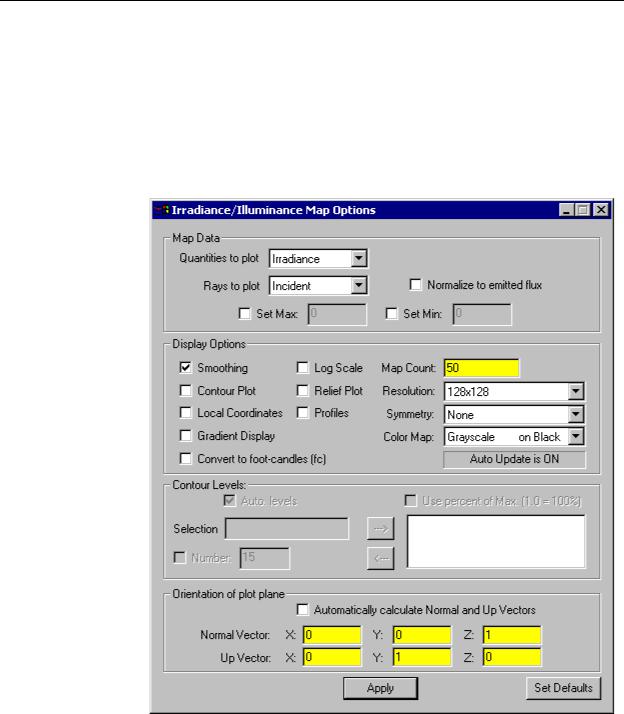
FIGURE 6.3 - Irradiance Options Dialog box

Irradiance map options are controlled through the Irradiance Options dialog box, accessed by selecting Analysis|Irradiance/Illuminance Options... or by right-clicking on the irradiance map and selection Irradiance/Illuminance Options... from the context menu. Each option and its function are described in the sections that follow.

TracePro 5.0 User’s Manual

6.5

Analysis

Map Data

The Map Data defines what quantities are displayed in the plot.

Quantities to Plot

Selects the map type to display. You can choose from:

•Irradiance, a plot of power per unit area of radiation incident on or absorbed by a surface,

•CIE (x, y), a plot of color in CIE xy coordinates,

•CIE (u’,v’), a plot of color in CIE u’v’ coordinates,

•True Color

Rays to Plot

You can observe a map of either absorbed or incident rays. Incident irradiance maps can be misleading when the selected surface is hit several times by the same ray. For example, a surface between two infinite parallel mirrors would have the same ray intersect the surface until the ray fell below the flux threshold or intercept threshold generating a incident flux many time greater that the starting flux of the ray.

Normalize

Normalize the map data to the total emitted flux from all sources.

This option allows you to have the flux and irradiance normalized to the total emitted flux. When this box is checked, TracePro divides the values in the irradiance map and the total flux by the emitted flux. This is especially useful for calculating system transmittance for an optical system, or lighting efficiency for a lighting calculation.

Example 1: System Transmittance

Suppose you need to calculate the system transmittance of an optical system. You would probably use the grid raytrace option, and the emitted flux is equal to the sum of the flux in all the emitted rays. When you display an irradiance map, the system transmittance is equal to the total flux, displayed at the bottom of the irradiance map window, divided by the emitted flux. To get the system transmittance, check the Normalize to emitted flux box and press the Apply button. The map will be redisplayed, and the Normalized Flux value will be equal to the system transmittance.

Example 2: Lighting Efficiency

Suppose you need to calculate the lighting efficiency of a luminaire in illuminating a plane. You would probably choose the Surface Source raytrace option, and the emitted flux is equal to the flux you specified when you defined the sources. When you display an irradiance map, the total flux incident on the observation plane is displayed at the bottom of the window. The lighting efficiency is equal to the total flux divided by the emitted flux. To get the lighting efficiency directly, check the Normalize to emitted flux box and press the Apply button. The map will be redisplayed, and the Normalized Flux value will be equal to the lighting efficiency of the luminaire.

6.6	TracePro 5.0 User’s Manual

Analysis Menu

Set Max/Min

The Max/Min values provide thresholds for the plot scale. If a Max value is set it will be used for the maximum value used in the irradiance plot. Any values which exceed the Max value will be displayed at the Max value. The Min value works in the same manner. If the Log Scale is set the Min value is disabled.

Display Options

The display options control the plot output.

Smoothing

If the smoothing box is checked, the irradiance distribution will be smoothed using a Gaussian smoothing kernel of the form

K(x, y)	1	–(x2 + y2) ⁄ (2σ2)	,	(6.1)
	= ------------e
	2πσ2

where σ is the waist radius of the Gaussian, taken as the Map Count value expressed in linear units. For example, the default value of 50 means that the waist radius of the kernel is 1/50 of the width of the map.

The smoothing is done by convolving this kernel with the irradiance distribution,

Esmooth(x, y) = ∫∫E(x', y')K(x – x', y – y')dx'dy'

(6.2)

The convolution is done by Fourier transforming, applying a filter, and inverse Fourier Transforming.

Contour Plot

Selecting Contour Plot creates a topographic map of the irradiance. Smoothing is always turned on when you select Contour Plot. The number of contours and contour levels is described in the Contour Levels section below.

Local Coordinates

The corners of the plot are labeled with coordinate data for the selected surface. By default the corners are labeled in global X, Y, Z points. Checking this item will display the corners in local X, Y coordinates.

Gradient Display

Checking this box causes a continuous gradation of colors to be displayed instead of discrete contours.

Convert to foot-candles

Scales plotted values to foot-candles.

Log Scale

Checking this box displays the irradiance on a logarithmic scale. This is especially useful when you need to see details in the very lowest irradiance values. This might be needed, for example, in a stray light analysis.

If you check Logarithmic Scale and Smoothing at the same time while also selecting a large number for Map Count (greater than 40), you can see artifacts in

TracePro 5.0 User’s Manual

6.7

Analysis

the display of the irradiance map in the form of cross-shaped patterns surrounding sharp peaks in the pattern. This is a result of aliasing and should be ignored.

Relief Plot

This option produces a 3D relief plot using OpenGL. See Figure 6.5 on page 6.9.

Profiles

Checking this box causes cross-sectional plots of the Irradiance/Illuminance to be displayed. When you press Apply, additional plots are shown that contain the profiles. To change the axes of inspection for the Profiles option, click a different point in the Irradiance/Illuminance map. A new set of horizontal and vertical axes are set at this point, and they are displayed in the profiles area of the window. Each profile passes through the point you selected with the mouse. Each time you select a new point, the display is updated. Clicking a point outside the Irradiance/ Illuminance map (but still inside the Irradiance/Illuminance map window) causes the profiles to become blank. To remove the profiles altogether, uncheck the Profiles check box and press Apply. See Figure 6.4 on page 6.9.

The vertical axis of the profile plot corresponds to the Irradiance/Illuminance scale. The horizontal axis corresponds to the linear size of the plotted area where the left hand side of the plot shows the position of the left side of the horizontal cursor line and the bottom position of the vertical cursor line. Two profile plots are drawn for the two cursor lines displayed.

Map Count

The count determines the resolution of the display on the irradiance map. The count value is the number of pixels in the irradiance map in both the horizontal and vertical directions. TracePro displays a square irradiance map and square pixels. Thus, while the width and height of the pixels are the same on the screen, their actual displacements may be different dependent on the range of values plotted in the two orthogonal directions. When Smoothing is enabled the map count is used to control the degree of smoothing applied to the data.

Resolution

Sets the size of the data grid for smoothing. The smoothing uses a Fast Fourier Transform (FFT) which requires a grid size of a power of 2.

Symmetry

Using this option you can take advantage of known symmetry on an irradiance or illuminance map. A smoother distribution can be obtained from fewer rays. The five symmetry selections are:

•None - This is the default where no symmetry is applied.

•Left / Right - Symmetry is applied between the left and right halves of the map.

•Up / Down - Symmetry is applied between the upper and lower halves of the map.

•Quadrant - This is the combination of Left / Right and Up / Down symmetry.

•Rotational - Symmetry is applied about an axis perpendicular to the center of the map.

The symmetry selection should be used with caution. TracePro will force symmetry onto the irradiance/illuminance map even if your model does not

6.8	TracePro 5.0 User’s Manual

Analysis Menu

possess symmetry. The user, through this option, conveys to TracePro that the data being plotted actually has the selected symmetry.

Color Map

Use this drop-down list to opt for either grayscale or one of several color-coded schemes. The choice of color affects both the display and the contour map display.

Surface boundary

Profile cursors and plot

FIGURE 6.4 - Irradiance Map with Profiles for Elliptical Reflector Demo

FIGURE 6.5 - Irradiance Map contours in 3D for Elliptical Reflector Demo

TracePro 5.0 User’s Manual

6.9