Analysis Menu

Candela Plots

Candela plots can be viewed by first selecting Analysis|Candela Plots and next selecting Polar Iso-Candela, Rectangular Iso-Candela, Polar Candela

Distribution or Rectangular Candela Distribution.

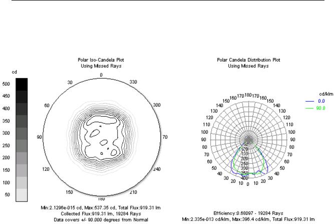
FIGURE 6.11 - Polar Iso Candela Contours (left) Candela Distribution in Luminaire Format (right)

A candela plot is a plot of luminous intensity, or flux per solid angle. In photometric units, a luminous intensity plot is in units of candelas (lumens per steradian). In radiometric units, an intensity plot is in units of watts per steradian. Candela plots are commonly used in the design of illumination systems, especially those used in the far field.

Candela data can be collected from ray sets of Missed rays, rays Exiting a surface or rays Incident on a surface. Missed rays are a collection of all rays that “leave” the model and “go off to infinity.” Exiting rays are the collection of ray segments following the intersection point of a ray at a surface. Due to ray splitting, several ray segments may contribute to the candela data for each incident ray. Incident rays are the collection of ray segments which intersect the selected surface. No surface selection is required for Missed rays but one is necessary for Exiting and Incident rays.

The candela plots represent flux versus angle and can be smoothed using the Candela Options dialog box. The iso-candela plots can be presented as false color maps or contour plots. The distribution plots are graphs of cross-sectional curves through the candela distribution.

The orientation of the candela plots is determined by the Normal Vector and the Up Vector, as specified in the Analysis|Candela Options dialog box. The normal vector specifies the axis of the candela plot and the up vector specifies “which way is up.”

TracePro 5.0 User’s Manual

6.17

Analysis

Candela Options

Candela map options are controlled through the Candela Options dialog box, accessed by selecting Analysis|Candela Options or by right-clicking on the candela plot. The dialog box is divided into tabbed tabs:

•Orientation and Rays

•Polar Iso-Candela

•Rectangular Iso-Candela

•Candela Distributions

FIGURE 6.12 - Candela Options dialog with the Orientation and Rays tab displayed.

The Orientation and Rays options section is used for all Candela plots. Each option and its function are described in the sections that follow.

Set Defaults

The options are saved when the Model is written to disk in an OML file. After the data is changed, pressing the Set Defaults button with stored the data into the TracePro defaults files to be used the next time TracePro is opened. See “User Defaults” on page 1.9.

6.18	TracePro 5.0 User’s Manual

Analysis Menu

Orientation and Rays

Normal Vector

The Normal Vector is a vector in 3D space that is used to orient the polar axis in candela plots. The center of the candela/intensity plots is based on that direction. On the map, the normal vector is pointing away from you and toward the candela plot. It as though are looking along the vector that is pointing to the center of the distribution, and the standard is to look along the direction of light propagation.

For example, if you are designing an illuminator that projects light to the right, i.e., along the +z axis, then you probably want the Normal Vector to be X=0, Y=0, Z=1.

Up Vector

The Up Vector is a vector in 3D space that is used to orient the direction that is “up” in the candela plots. The orientation is defined so that the Up Vector points up, i.e. toward the top of the screen in the candela plots. For example, if you are designing an illuminator that projects light to the right as in the example described in the previous paragraph, i.e., along the +z axis, then you probably want the Normal Vector to be X=0, Y=0, Z=1. Since the y axis normally points up in TracePro, you probably want the Up Vector to be X=0, Y=1, Z=0 for this example. If you want to see what that distribution would look like if you were standing on your head, set the Up Vector to X=0, Y=-1, Z=0.

Candela Plot Orientation Example

For example, if you are designing an illuminator that projects light to the right, i.e., along the +z axis, then you probably want the Normal Vector to be X=0, Y=0, Z=1. Since the y axis normally points up in TracePro, you probably want the Up Vector to be X=0, Y=1, Z=0 for this example. If you are designing a light fixture that points down, then you want the normal vector to be X=0, Y=-1, Z=0 and the Up Vector to be either X=1, Y=0, Z=0 or X=0, Y=0, Z=1. Figure 6.13 shows two hemispheres that correspond to the Normal and Up vectors defined in this example. The picture on the left has a Normal of (0,0,1) and the picture on the right has a normal of (0,- 1,0). The Normal and Up vectors reference the global origin displayed in Figure 6.13.

FIGURE 6.13 - Candela hemispheres for left) Normal vector (0,-1,0), Up vector (0,0,1) and right) Normal vector (0,0,1), Up vector (0,1,0)

TracePro 5.0 User’s Manual

6.19

Analysis

Ray Selection

Ray Selection lets you choose which rays to use as Candela Data. You can select either missed rays, exiting rays from a selected surface, or incident rays from a selected surface.

Data Processing | Symmetry

Using this option, you can take advantage of known symmetry on a Candela plot. A smoother distribution can be obtained from fewer rays. The five symmetry selections are:

•None - This is the default where no symmetry is applied.

•Left / Right - Symmetry is applied between the left and right halves of the plot.

•Up / Down - Symmetry is applied between the upper and lower halves of the plot.

•Quadrant - This is the combination of Left / Right and Up / Down symmetry.

•Rotational - Symmetry is applied about an axis perpendicular to the center of the plot.

The symmetry selection should be used with caution. TracePro will force symmetry onto the Candela plot even if your model does not possess symmetry. The user, through this option, conveys to TracePro that the data being plotted actually has the selected symmetry.

Polar Iso-Candela

A Polar Iso-Candela Plot shows spherical polar angle on the polar axis. It shows a spherical azimuth angle in the azimuth direction. This plot maps a hemisphere onto a plane. The distribution plots display curves in either rectangular or polar format.

6.20	TracePro 5.0 User’s Manual

Analysis Menu

FIGURE 6.14 - Candela Options dialog with the Polar Iso-Candela tab displayed.

Smoothing

If the smoothing box is checked, the intensity distribution will be smoothed using a Gaussian smoothing kernel of the form

K(θx, θy)	1	–(θx2 + θy	2) ⁄ (2σ2)	,	(6.3)
	= ------------e
	2πσ2

where σ is the waist radius of the Gaussian. The number to the right of the Smoothing check box is used as the waist radius. For example, a value of 20 means that the waist radius of the kernel is 1/20 of the width of the map.

The smoothing is done by convolving this kernel with the candela or intensity distribution,

Esmooth(θx, θy) = ∫∫E(θx', θy')K(θx – θx', θy – θy')dθx'dθy' , (6.4)

The convolution is done by Fourier transforming, applying a filter, and inverse Fourier transforming.

Contour Plot

If the Contour Plot box is checked, the Polar Iso-Candela data is displayed as a contour plot. The number of levels displayed is determined by the Number entry in the Levels part of the Polar Plots section of the dialog box.

TracePro 5.0 User’s Manual

6.21