Defining Sources

Table 5.3 lists the Wavelength data of a Grid Source. You can enter wavelengths and weights, while flux and number of rays are determined by entries on the Grid Setup tab.

TABLE 5.3. Grid Source Options - Wavelength

	Wavelength tab
Attribute		Value(s)
Wavelength		Discrete wavelength(s) in μm. Add wave-
		lenths by typing the wavelength, and click-
		ing Add or typing the Enter key. Delete
		wavelength(s) by selecting them in the
		table and clicking Delete.
Weight		Relative weighting factor to be applied to
		the flux for each wavelength.
Flux		Flux to emitted for this wavelength, a cal-
		culated value. For Total Flux or Total Irra-
		diance sources, the flux for each
		wavelength will be adjusted so that they
		add up to the total flux as determined by
		the Flux or Irradiance entry on the Grid
		Setup tab.
#Rays		Calculated, depending on choices on Grid
		Setup tab. For Random grid pattern, the
		number of rays for each wavelength will
		adjusted so that the flux per ray for each
		wavelength is approximately the same.

The Polarization tab provides a means to set the initial Polarization state of the rays emitted from the Grid plane. The polarization options are listed in Table 5.4.

TABLE 5.4. Grid Source Options - Polarization Setup

Standard Expert	Polarization tab
Attribute	Value(s)
Polarization state	Unpolarized, linear, circular, or custom
Degree of Polarization	0 < degree <= 1
Custom Polarization	Method, Handedness, Ratio, Orientation
Normalized Stokes Vector	Display only

Once you have set the parameters, click the Trace This button and the raytrace begins. See “Standard (Forward) Raytrace” on page 5.28

Setting Up the Grid

Grid Boundary

The grid boundary specifies the shape and dimensions of the boundary within which a planar grid of rays is generated. Rays are generated according to the grid pattern. Ray starting points that are outside the grid boundary are truncated, thus,

TracePro 5.0 User’s Manual

5.7

Ray Tracing

the total number of rays actually traced may not agree with the total number provided in the dialog box. Grid patterns and boundaries can be mixed and matched.

Shape

An annular grid boundary means that an annulus is defined with radii given by the grid dimensions. All ray starting points are required to lie within the annulus.

For example, if a rectangular Grid Pattern is chosen with an annular grid boundary, rays are started in a square grid with sides equal to the outer diameter of the annulus. Points outside the annulus—in the hole of the annulus or in the corners of the square—are eliminated.

If a rectangular grid boundary is used with a circular grid pattern, then the diagonal dimension of the rectangular boundary is used as the diameter of the circular grid. Points in the circle that lie outside the rectangle are truncated.

If an annular grid boundary is used with a circular grid pattern, rays in the hole of the annulus are truncated.

If a random grid is chosen, points are randomly selected within the boundary (either annular or rectangular).

Dimensions

• Outer Radius or Y Half-Height of Grid

Outer radius refers to the outer radius of the annular boundary. The y half-height is the half-height of the rectangular grid boundary in the direction of the Up vector or local y-axis of the grid.

• Inner Radius or X Half-Width of Grid

Inner radius refers to the inner radius of the annular boundary. Inner radius is the half-width of the rectangular grid boundary in the local x direction of the grid.

Grid Pattern

Regular and dithered grids are defined by an array of cells. Once the grid pattern is chosen, the area surrounded by the grid boundary is divided into an array of cells, each with equal area. Then one ray is started from within each cell. For circular, rectangular, and cross grids, each ray is started from the geometric center of each cell. In a dithered rectangular grid, for each cell a point is chosen at random within the cell, and a ray is started from that point.

For a random grid, the grid boundary is not subdivided and each ray is started from a totally random location within the grid boundary.

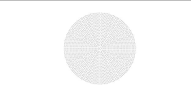
Circular

In a circular grid pattern, rays are started in rings. The first ring is simply a point at the center of the circle, and the second ring consists of six rays equally spaced around a circle. Each successive ring has an additional six rays. The radii of the rings are set so that each ray represents an equal area.

If you choose a number of rings equal to n, the number of rays N that are generated is:

N = 3n(n – 1) + 1

(5.1)

5.8	TracePro 5.0 User’s Manual

Defining Sources

FIGURE 5.4 - Example of circular grid with 25 rings resulting in 1801 rays

Rectangular

In a rectangular grid pattern, rays start in a rectangular pattern, spaced in equal increments along each of the local x and y-axes. To determine the starting points for the rays, the boundary region is divided into rectangular cells.

For a rectangular boundary, the rectangle is divided into Nx x Ny cells, where Nx and Ny are the number of points in the local or grid x and y directions,

respectively. The local x and y directions are determined by the Grid Orientation at the bottom of the dialog box.

For an annular region, a square with side equal to the diameter of the outer circle is used for the boundary region. Once the cells are determined, one ray is started from the center of each cell. That results in a regularly spaced grid of rays.

The spacing of the ray starting points need not be the same in the x and y directions. In other words, the cells for determining the ray starting points need not be square, but are rectangular in general. The grid spacing (or cell aspect ratio) is determined by the aspect ratio of the boundary and the values of Nx and Ny.

TracePro 5.0 User’s Manual

5.9

Ray Tracing

FIGURE 5.5 - Example of rectangular grid with Nx = 50 and Ny = 50 and a square boundary, resulting in a square pattern with 2500 rays.

Dithered

Dithering is a process by which the rays in a rectangular grid are altered slightly to introduce randomness in their starting positions—a compromise between a rectangular grid and a random grid. Dithering breaks up pattern noise that occurs with a rectangular grid while avoiding holes and clumps that occur in a random grid.

The dithering is accomplished in TracePro by first defining a rectangular array of cells as for the rectangular ray grid, then choosing a ray starting point randomly within each cell.

The cells for determining the ray starting points for a dithered grid need not be square, but are rectangular in general. The cell aspect ratio is determined by the aspect ratio of the boundary and the values of Nx and Ny.

5.10	TracePro 5.0 User’s Manual

Defining Sources

FIGURE 5.6 - Example of a dithered rectangular grid with Nx = 50 and Ny =

50 and a square boundary. Compare this with the figures for a rectangular grid (Figure 5.5) and for a random grid (Figure 5.8).

Cross

The cross grid pattern lets you generate two lines of rays, one in the horizontal direction, the other in the vertical direction. The number of rays in each direction is always an odd number, so that there is always a ray at the center of the pattern. If you enter an even number, one will be added to it to obtain an odd number before the rays are generated. The ray starting points are determined by dividing the boundary region into a grid of rectangular cells numbering Nx x Ny.

The cells for determining the ray starting points need not be square, but are rectangular in general. The cell aspect ratio is determined by the aspect ratio of the boundary and the values of Nx and Ny.

FIGURE 5.7 - Example of Cross grid with Nx = 50 and Ny = 50 resulting in a pattern of 101 rays.

Random grid

In a random grid, points are selected randomly within the grid boundary. For a rectangular boundary, points are selected at random within the rectangle, and for

TracePro 5.0 User’s Manual

5.11

Ray Tracing

an annular boundary, they are selected randomly within the annulus. Instead of choosing the Nx and Ny values or a number of rings, you directly enter the total

number of rays to be traced.

A random grid is the purest form of Monte Carlo simulation, though it is not necessarily the best. As can be seen in Figure 5.8, especially when contrasted with the dithered random grid of Figure 5.6, the random distribution suffers from voids and clumps in the ray distribution. This is bothersome if your model contains a small design detail that needs a good sampling of rays (that is, not overor under-sampling)

FIGURE 5.8 - Example random grid pattern with 2500 rays and a square boundary. Compare this with the figures for a rectangular grid and for a dithered rectangular grid (above).

Checkerboard

This pattern includes major and minor increments for the ray positions within the pattern. Between each major point additional rays will be traced for each set of minor points. The new dialog is shown in Figure 5.9.

5.12	TracePro 5.0 User’s Manual

Defining Sources

FIGURE 5.9 - Grid Source with checkerboard pattern

The output from the above ray grid is shown as an irradiance plot in Figure 5.10.

FIGURE 5.10 - Irradiance plot showing checkerboard grid pattern

TracePro 5.0 User’s Manual

5.13