

- •User’s Manual
- •COPYRIGHT
- •TRADEMARKS
- •LICENSE AGREEMENT
- •WARRANTY
- •DOCUMENT CONVENTIONS
- •What is TracePro?
- •Why Solid Modeling?
- •How Does TracePro Implement Solid Modeling?
- •Why Monte Carlo Ray Tracing?
- •The TracePro Graphical User Interface
- •Model Window
- •Multiple Models in Multiple Views
- •System Tree Window
- •System Tree Selection
- •Context Sensitive Menus
- •Model Window Popup Menus
- •System Tree Popup Menus
- •User Defaults
- •Objects and Surfaces
- •Changing the Names
- •Selecting Objects, Surfaces and Edges
- •Moving Objects and Other Manipulations
- •Interactive Viewing and Editing
- •Normal and Up Vectors
- •Modeling Properties
- •Applying Properties
- •Modeless Dialog Boxes
- •Expression Evaluator
- •Context Sensitive OnLine Help
- •Command Line Arguments
- •Increasing Access to RAM on 32-bit Operating Systems
- •Chinese Translations for TracePro Dialogs
- •Introduction to Solid Modeling
- •Model Units
- •Position and Rotation
- •Defining Primitive Solid Objects
- •Block
- •Cylinder/Cone
- •Torus
- •Sphere
- •Thin Sheet
- •Rubberband Primitives
- •Defining TracePro Solids
- •Lens Element
- •Lens tab
- •Aperture tab
- •Obstruction tab
- •Position tab
- •Aspheric tab
- •Fresnel Lens
- •Reflector
- •Conic
- •3D Compound
- •Parabolic Concentrators
- •Trough (Cylinder)
- •Compound Trough
- •Rectangular Concentrator
- •Facetted Rim Ray
- •Tube
- •Baffle Vane
- •Boolean Operations
- •Intersect
- •Subtract
- •Unite
- •Moving, Rotating, and Scaling Objects
- •Translate
- •Move
- •Rotate
- •Scale
- •Orientation
- •Sweeping and Revolving Surfaces
- •Sweep
- •Revolve
- •Notes Editor
- •Importing and Exporting Files
- •Exchanging Files with Other ACIS-based Software
- •Importing an ACIS File
- •Exporting an ACIS File
- •Stereo Lithography (*.STL) Files
- •Additional CAD Translators (Option)
- •Plot formats for model files
- •Healing Imported Data
- •How to Autoheal an Object
- •How to Manually Heal an Object
- •Reverse Surfaces (and Surface Normal)
- •Combine
- •Lens Design Files
- •Merging Files
- •Inserting Files
- •Changing the Model View
- •Silhouette Accuracy
- •Zooming
- •Panning
- •Rotating the View
- •Named Views
- •Previous View
- •Controlling the Appearance of Objects
- •Display Object
- •Display All
- •Display Object WCS
- •Display RepTile
- •Display Importance
- •Customize and Preferences
- •Preferences
- •Customize
- •Changing Colors
- •Overview
- •What is a property?
- •Define or Apply Properties
- •Property Editors
- •Toolbars and Menus
- •Command Panel
- •Information Panel
- •Grid Panel
- •Material Properties
- •Material Catalogs
- •Material Property Database
- •Create a new material property
- •Editing an existing material property
- •Exporting a material property
- •Importing a Material Property
- •Bulk Absorption
- •Birefringence
- •Bulk Scatter Properties
- •Bulk Scatter Property Editor
- •Import/Export
- •Scatter DLL
- •Fluorescence Properties
- •Defining Fluorescence Properties
- •Fluorescence Calculations
- •Fluorescence Ray Trace
- •Raytrace Options
- •Surface Source Properties
- •Surface Source Property Editor
- •Create a New Surface Source Property
- •Edit an Existing Surface Source Property
- •Export a Surface Source Property
- •Import a Surface Source Property
- •Gradient Index Properties
- •Gradient Index Property Editor
- •Create a New Gradient Index Property
- •Edit an Existing Gradient Index Property
- •Export a Gradient Index Property
- •Import a Gradient Index Property
- •Surface Properties
- •Using the Surface Property Database
- •Using the Surface Property Editor
- •Using Solve for
- •Direction-Sensitive Properties
- •Creating a new surface property
- •Editing an Existing Surface Property
- •Exporting a Surface Property
- •Importing a Surface Property
- •Surface Property Plot Tab
- •Incident Medium
- •Substrate Medium
- •by angle (deg)
- •by wavelength (um)
- •Display Values
- •Table BSDF
- •Creating a Table BSDF Property
- •Creating an Asymmetric Table BSDF Property
- •Using an Asymmetric Table BSDF property
- •Wire Grid Polarizers
- •Upgrading an older property database
- •Applying Wire-Grid Surface Properties
- •Thin Film Stacks
- •Using the Stack Editor
- •Thin Film Stack Editing Note
- •Entering a Single Layer Stack
- •RepTile Surfaces
- •Overview
- •Specifying a RepTile surface
- •RepTile Shapes
- •RepTile Geometries
- •RepTile Parameterization
- •Variables
- •Parameterized Input Fields
- •Decentering RepTile Geometry
- •Property Database Tools
- •Import
- •Export
- •Using Properties
- •Limitations in Pre-Defined Property Data
- •Applying Property Data
- •Material Properties
- •Material Catalogs
- •Applying Material Properties
- •Applying Birefringent Material Properties
- •Bulk Scattering
- •Fluorescence Properties
- •Applying Fluorescence Properties
- •Gradient Index Properties
- •Surface Properties
- •Using the Surface Property Database
- •Surface Source Properties
- •Blackbody Surface Sources
- •Blackbody and Graybody Calculations
- •Source Spreadsheet
- •Scaling the Total Rays for Several Sources
- •Prescription
- •Color
- •Importance Sampling
- •Defining Importance Sampling Targets (Manually)
- •Adding Targets
- •Number of Importance Rays
- •Shape, Dimensions, and Location of Importance Targets
- •Cells
- •Apply the Importance Sampling Property
- •Automatic Setup of Importance Sampling
- •Define the Prescription
- •Select the Target Shape
- •Apply, Cancel, or Save Targets
- •Editing/Deleting Importance Sampling Targets
- •Exit Surface
- •Predefined irradiance map orientation
- •Diffraction
- •Defining Diffraction in TracePro
- •Do I need to Model Diffraction in TracePro?
- •How do I Set Up Diffraction?
- •Using the Raytrace Flag
- •Mueller Matrix
- •Temperature
- •Class and User Data
- •RepTile Surfaces
- •Overview
- •Specifying a RepTile surface
- •Boundary Shapes
- •Export
- •Visualization and Surface Properties
- •Specifying a RepTile Texture File Surface
- •Bump Designation for Textured RepTile
- •Base Plane Designation for Textured RepTile
- •Temperature Distribution
- •Introduction to Ray Tracing
- •Combining Sources
- •Managing Sources with the System Tree
- •Managing Sources with the Source/Wavelength Selector
- •Defining Sources
- •Grid Sources
- •Setting Up the Grid
- •Grid Density: Points/Rings
- •Beam Setup
- •Wavelengths
- •Polarization
- •Surface Sources
- •Importance Sampling from Surface Sources
- •File Sources
- •Creating a File Source from Radiant Imaging Data
- •Creating a File Source from an Incident Ray Table
- •Creating a File Source from Theoretical or Measured Data
- •Insert Source
- •Capability to “trace every nth ray”
- •Capability to scale flux
- •Modify the File Source
- •Orienting and Selecting Sources
- •Multi-Selecting Sources
- •Move and Rotate Dialogs
- •Tracing Rays
- •Standard (Forward) Raytrace
- •Reverse Ray Tracing
- •Specifying reverse rays
- •Theory of reverse ray tracing
- •Luminance/Radiance Ray Tracing
- •Raytrace Options
- •Options
- •Analysis Units
- •Ray Splitting
- •Specular Rays Only
- •Importance Sampling
- •Aperture Diffraction and Aperture Diffraction Distance
- •Random Rays
- •Fluorescence
- •Polarization
- •Detect Ray Starting in Bodies
- •Random Seed
- •Wavelengths
- •Thresholds
- •Simulation and Output
- •Collect Exit Surface Data
- •Collect Candela Data
- •Index file name
- •Save Data to Disk during Raytrace
- •Save Ray History to disk
- •Sort Ray Paths
- •Save Bulk Scatter data to disk
- •Simulation Options for TracePro LC
- •Collect Exit Surface Data
- •Collect Candela Data
- •Advanced Options
- •Voxelization Type
- •Voxel Parameters
- •Raytrace Type
- •Gradient Index Substep Tolerance
- •Maximum Nested Objects
- •Progress Dialog
- •Ray Tracing modes
- •Analysis Mode
- •Saving and Restoring a Ray-Trace
- •Simulation Mode
- •Simulation Dialog
- •Simulation Options
- •Simulation Data for LC
- •Examining Raytrace Results
- •Analysis Menu
- •Display Rays
- •Ray Drawing Options
- •Ray Colors
- •Flux-based ray colors
- •Wavelength-based ray colors
- •Source-based ray colors
- •All rays one color
- •Irradiance Maps
- •Irradiance Map Options
- •Map Data
- •Display Options
- •Contour Levels
- •Access to Irradiance Data
- •Ensquared Flux
- •Luminance/Radiance Maps
- •3D Irradiance Plot
- •Candela Plots
- •Candela Options
- •Orientation and Rays
- •Polar Iso-Candela
- •Rectangular Iso-Candela
- •Candela Distributions
- •IESNA and Eulumdat formats
- •Access to Candela/Intensity Data
- •Enclosed Flux
- •Polarization Maps
- •Polarization Options
- •Save Polarization Data
- •OPL/Time-of-flight plot
- •OPL/Time-of-flight plot options
- •Incident Ray Table
- •Copying and Pasting the Incident Ray Table Data
- •Saving the Incident Ray Table in a File
- •Saving the Incident Ray Table as a Source File
- •Display Selected Rays
- •Source Files - Binary file format
- •Ray Histories
- •Copying and Pasting the Ray History Table Data
- •Saving the Ray History Table in a File
- •Ray Sorting
- •Ray Sorting Examples
- •Reports Menu
- •Flux Report
- •Property Data Report
- •Raytrace Report
- •Saving and Restoring a Raytrace
- •Tools Menu
- •Audit
- •Delete Raydata Memory
- •Collect Volume Flux
- •Overview
- •View Volume Flux
- •Overview
- •Flux Type
- •Normal Axis/Orientation
- •Slices
- •Color Map
- •Gradient
- •Logarithmic
- •Simulation File Manager
- •Irradiance/Illuminance Viewer
- •Overview
- •Viewing a saved Irradiance/Illuminance Map
- •Irradiance/Illuminance Viewer Options
- •Adding and Subtracting Irradiance/Illuminance Maps
- •Measurement Dialog
- •Introduction
- •The Use of Ray Splitting in Monte Carlo Simulation
- •Importance Sampling
- •Importance Sampling and Random Rays
- •When Do I Need Importance Sampling?
- •How to Choose Importance Sampling Targets
- •Importance Sampling Example
- •Material Properties
- •Material Property Database
- •Material Property Interpolation
- •Gradient Index Profile Polynomials
- •Complex Index of Refraction
- •Surface Properties
- •Coincident Surfaces
- •BSDF
- •Harvey-Shack BSDF
- •ABg BSDF Model
- •BRDF, BTDF, and TS
- •Elliptical BSDF
- •What is an elliptical BSDF?
- •Elliptical ABg BSDF model
- •Elliptical Gaussian BSDF
- •Calculation of Fresnel coefficients during raytrace
- •Anisotropic Surface Properties
- •Anisotropic surface types
- •Getting anisotropic data
- •User Defined Surface Properties
- •Overview
- •Creating a Surface Property DLL
- •Create the Surface Property
- •Apply Surface Property
- •API Specification for Enhanced Coating DLL
- •Document Layout
- •Calling Frequencies
- •Return Codes, Signals, and Constants -- TraceProDLL.h
- •Description of Return Codes
- •Function: fnInitDll
- •Function: fnEvaluateCoating
- •Function: fnAnnounceOMLPath
- •Function: fnAnnounceDataDirectory
- •Function: fnAnnounceSurfaceInfo
- •Function: fnAnnounceLocalBoundingBox
- •Function: fnAnnounceRaytraceStart
- •Function: fnAnnounceWavelengthStart
- •Function: fnAnnounceWavelengthFinish
- •Function: fnAnnounceRaytraceFinish
- •Example of Enhanced Coating DLL
- •Surface Source Properties
- •Spectral types
- •Rectangular
- •Gaussian
- •Solar
- •Table
- •Angular Types
- •Lambertian
- •Uniform
- •Gaussian
- •Solar
- •Table
- •Mueller Matrices and Stokes Vectors
- •Bulk Scattering
- •Henyey-Greenstein Phase Function
- •Gegenbauer Phase Function
- •Scattering Coefficient
- •Using Bulk Scattering in TracePro
- •User Defined Bulk Scatter
- •Using Scatter DLLs
- •Required DLL Functions called from TracePro
- •Common Arguments passed from TracePro
- •DLL Export Definitions
- •Non-Uniform Temperature Distributions
- •Overview
- •Distribution Types
- •Rectangular Coordinates
- •Circular Coordinates
- •Cylindrical Coordinates
- •Defining Temperature Distributions
- •Format for Temperature Distribution Storage Files
- •Type 0: Rectangular with Interpolated Points
- •Type 1: Rectangular with Polynomial Distribution
- •Type 2: Circular with Interpolated Points
- •Type 3: Circular with Polynomial Distribution
- •Type 4: Cylinder with Interpolated Points
- •Type 5: Cylinder with Polynomial Distribution
- •Polynomial Approximations of Temperature Distributions
- •Interpretation of Polar Iso-Candela Plots
- •Property Import/Export Formats
- •Material Property Format
- •Surface Property Format
- •Surface Data Columns
- •Grating Data Columns
- •Stack Property Format
- •Gradient Index Property Format
- •Gradient Index Data Columns (non-GRADIUM types)
- •Gradient Index Data Columns (GRADIUM (Buchdahl) type)
- •Gradient Index Data Columns (GRADIUM (Sellmeier) type)
- •Bulk Scatter Property Format
- •Fluorescence Property Format
- •Surface Source Property Format
- •RepTile Property Format
- •Texture File Format
- •The Scheme Language
- •Scheme Editor
- •Overview
- •Text Color
- •Macro Recorder
- •Recording States
- •Macro Format and Example
- •Macro Command Examples
- •Running a Macro Command from the Command Line
- •Running a Scheme Program Stored in a File
- •Scheme Commands
- •Creating Solids
- •Create a solid block:
- •Create a solid block named blk1:
- •Create a solid cylinder:
- •Create a solid elliptical cylinder:
- •Create a solid cone:
- •Create a solid elliptical cone:
- •Create a solid torus:
- •Boolean Operations
- •Boolean subtract
- •Boolean unite
- •Boolean intersect
- •Chamfers and blends
- •Macro Programs
- •Accessing TracePro Menu Selections using Scheme
- •For more information on Scheme
- •TracePro DDE Interface
- •Introduction
- •The Service Name
- •The Topic
- •The Item
- •Clipboard Formats
- •TracePro DDE Server
- •Establishing a Conversation
- •Excel 97/2000 Example
- •RepTile Examples
- •Fresnel lens
- •Conical hole geometry with variable geometry, rectangular tiles and rectangular boundary
- •Parameterized spherical bump geometry with staggered ring tiles
- •Aperture Diffraction Example
- •Applying Importance Sampling to a Diffracting Surface
- •Volume Flux Calculations Example
- •Sweep Surface Example
- •Revolve Surface Example
- •Using Copy with Move/Rotate
- •Example of Orienting and Selecting Sources
- •Creating the TracePro Source Example OML
- •Moving and Rotating the Sources from the Example
- •Anisotropic Surface Property
- •Creating an anisotropic surface property in TracePro
- •Applying an anisotropic surface property to a surface
- •Elliptical BSDF
- •Creating an Elliptical BSDF property
- •Applying an elliptical BSDF surface property to a surface
- •Using TracePro Diffraction Gratings
- •Using Diffraction Gratings in TracePro
- •Ray-tracing a Grating Surface Property
- •Example Using Reverse Ray Tracing
- •Specifying reverse rays
- •Setting importance-sampling targets
- •Tracing Reverse Rays
- •Viewing Analysis Results
- •Example using multiple exit surfaces
- •Example Using Luminance/Radiance Maps
- •Index

Interpretation of Polar Iso-Candela Plots
c1,7 c2,7 c3,7 c4,7 c5,7 c0,8 c1,8 c2,8 c3,8 c4,8 c5,8 c0,9 c1,9 c2,9 c3,9 c4,9 c5,9 c0,10 c1,10 c2,10 c3,10 c4,10 c5,10
z
[0.5 ( -1 + 3z2 )] [0.5 ( -3z + 5z3 )]
[0.125 ( 3 – 30z2 + 35z4 )] [0.125 ( 15z – 70z3 + 63z5 )] 1
z
[0.5 ( -1 + 3z2 )] [0.5 ( -3z + 5z3 )]
[0.125 ( 3 – 30z2 + 35z4 )] [0.125 ( 15z – 70z3 + 63z5 )] 1
z
[0.5 ( -1 + 3z2 )] [0.5 ( -3z + 5z3 )]
[0.125 ( 3 – 30z2 + 35z4 )] [0.125 ( 15z – 70z3 + 63z5 )] 1
z
[0.5 ( -1 + 3z2 )] [0.5 ( -3z + 5z3 )]
[0.125 ( 3 – 30z2 + 35z4 )] [0.125 ( 15z – 70z3 + 63z5 )]
cos4θ
cos4θ
cos4θ
cos4θ
cos4θ
sin4θ
sin4θ
sin4θ
sin4θ
sin4θ
sin4θ
cos5θ
cos5θ
cos5θ
cos5θ
cos5θ
cos5θ
sin5θ
sin5θ
sin5θ
sin5θ
sin5θ
sin5θ
Interpretation of Polar Iso-Candela Plots
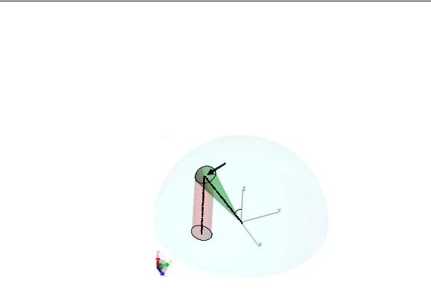
Iso-candela intensity plots (i.e., W/sr or cd depending on the units) can cause confusion to users. This section addresses such potential confusion by providing an example that illustrates what happens when you project a hemispherical distribution onto a plane. Figure 7.20 shows the sphere over which the intensity distribution should be viewed, and then how it is projected to the base plane of this hemisphere. For this simple illustration the projected solid angle is given by
dΩ = dωcosθ |
(7.45) |
where is the angle with respect to the normal axis, is the solid angle, and |
is the |
projected solid angle. In TracePro the angle is the one with respect to the |
|
Normal (as defined in Analysis|Candela Plot Options). Each of the rays is binned within constant solid angle bins (i.e., they span the same surface are on the unit hemisphere). Additionally, for Polar Iso-Candela plots, individually each
TracePro 5.0 User’s Manual |
7.81 |
Technical Reference
ray is corrected for the nonlinear projection from this hemisphere to the plane. This nonlinear projection is due to the constant angular spacing in the radial direction on polar iso-candela plots, as shown in Figure 7.21 and Figure 7.22 (i.e., the annular pie slices do not have constant areas as function of the radiant angle). Thus, two rays at different angles that are in the same bin with the same flux will contribute different amounts of intensity (cd or W/sr) to this bin. If you save the Polar Iso-candela data (File|Save As… of type *.txt), the nonlinear projection is also saved.
dω
θ
 dΩ
dΩ
FIGURE 7.20 - Depiction of solid angle projection from a hemisphere to the base plane of the hemisphere.
To illustrate this, consider the case shown in Figure 7.21, there are grid sources comprised each of single rays. Grid 1 has a ray in the x-z plane at an angle of 63.426º to the z axis. Grid 2 has a ray in the x-z plane at an angle of 64.537º to the z axis. Figure 7.22 shows the iso-candela plots (Analysis|Candela Plots|Polar Iso-Candela) for (a) Grid 1 and (b) Grid 2. Note the difference in the maximum candela values, which arises due to the nonlinear projection. Polar iso-candela plots in direction cosine values do not suffer from this projection effect since the cos(q) value in See Equation 7.45 on page 7.81 is simply the axial plot dimension. However such plots are currently not available in TracePro.
Finally, one can rotate the plot normal, by, for example, placing the Grid 1 ray at the pole. This is done by changing Analysis|Candela Plot Options > Orientation and Rays tab X to 0.8944 and Z to 0.4472. Figure 36 shows the results for (a) Grid 1 and (b) Grid 2.
7.82 |
TracePro 5.0 User’s Manual |

Interpretation of Polar Iso-Candela Plots
FIGURE 7.21 - Polar Iso-Candela Plots for Grids (a) 1 and (b) 2, Normal = (0, 0, 1).
FIGURE 7.22 - Polar Iso-Candela Plots for Grids (a) 1 and (b) 2, Normal = (0.8944, 0, 0.4472).
TracePro 5.0 User’s Manual |
7.83 |