Defining TracePro Solids

Reflector

The Insert|Reflector menu or Insert Reflector toolbar button opens a modeless dialog box that allows you to specify a reflector such as for a lamp or concentrator. The Insert Reflector dialog is a tabbed dialog box with six tabs for entering six different classes of reflectors and concentrators:

•Conic

•3D Compound

•Trough (Cylinder)

•Compound Trough

•Rectangular Concentrator

•Facetted Rim Ray

A reflector consists of a curved piece of material with the thickness and shape specified in the dialog box. The sections below describe each class of reflector.

Conic

A conic reflector is a conic section of revolution, i.e., one of the following:

•Spherical

•Parabolic

•Elliptical

•Hyperbolic

FIGURE 2.14 - Elliptical reflector with a hole at (0,0,0)

TracePro 5.0 User’s Manual

2.15

Creating a Solid Model

This dialog box allows you to specify the basic shape of the reflector (one of the above choices) as well as the focal length(s) or radius, as appropriate. You also specify the thickness, radius of a hole at the vertex, and the location and orientation of the reflector. A reflector specified with no rotation will be created in the orientation shown in Figure 2.14, with its axis of symmetry parallel to the z- axis, and the open end facing along the +z-axis.

Figure 2.14 shows an elliptical reflector with a hole at the vertex and located at the origin. The X, Y and Z coordinates of the origin serve to locate the vertex of the reflector. If you do not need a hole at the vertex, leave the hole radius set to zero.

FIGURE 2.15 - Insert Conic Reflector Dialog

The parameters necessary to specify a conic reflector are:

•Shape (e.g. circular, elliptical, etc.)

•Length (the distance from the vertex to the end of the reflector)

•Diameter

•Radius of curvature (spherical)

•Focal length(s) (non spherical)

•Thickness

•Hole radius (radius of an optional hole at the vertex)

2.16	TracePro 5.0 User’s Manual

Defining TracePro Solids

•Origin (X, Y, Z coordinates of the vertex)

•Rotation (X, Y, Z rotation angles about the vertex)

The length, diameter and radius/focal length(s) are related and you can select one value to be calculated using the Calculate drop down list and enter the others. For example, if you need a parabolic reflector to fit inside a known volume you can enter the length and diameter. Similarly, if you know the diameter and focal length you can calculate the length.

3D Compound

A 3D Compound reflector is a 3D compound concentrator. You can use this tab to make a:

•CPC (Compound Parabolic Concentrator),

•CEC (Compound Elliptical Concentrator)

This dialog tab actually allows you to make toroids formed from parabolas and ellipses, special cases of which are CPCs and CECs. You enter the axis tilt, lateral shift, and length of the concentrator independently, so that you can create shapes other than ideal CPCs and CECs. To create ideal CPCs and CECs, you must solve for one of these parameters in terms of the others yourself, then enter the result in the dialog.

The parameters necessary to specify a 3D Compound Reflector are:

•Shape (Elliptical or Parabolic)

•Front length (the distance from the focal points to the entrance port end of the concentrator)

•Back length (the distance from the focal points to the exit port end of the concentrator)

•Lateral focal shift (equal to the exit port radius for a textbook concentrator)

•Thickness

•Axis tilt (equal to the acceptance angle for a textbook concentrator)

•Focal length(s)

•Origin (X, Y, Z coordinates of the center of the exit port)

•Rotation (X, Y, Z rotation angles about the center of the exit port)

Note: A Conic Reflector is a special case of a 3D Compound Reflector. You could make a Conic Reflector by setting the Axis tilt and the Lateral focal shift to zero in the 3D Compound Reflector dialog tab.

For more information on concentrators, see the textbook: High Collection Nonimaging Optics, W.T. Welford and R. Winston, Academic Press, New York, 1989, ISBN 0-12-742885-2.

Parabolic Concentrators

A Compound Parabolic Concentrator (CPC) can be thought of as a parabolic toroid, i.e. a parabola revolved about an axis other than its axis of symmetry. A parabolic concentrator can be constructed by starting with a parabola, tilting it (about its focal point), displacing it laterally, then revolving it about its original axis of symmetry to form a surface.

TracePro 5.0 User’s Manual

2.17

Creating a Solid Model

A CPC is the best theoretical shape for concentration of light from a distant source when the parameters are chosen as described in Welford and Winston. TracePro also allows you to enter a CPC that is not an optimal concentrator surface.

In TracePro, the shape of a CPC is described by the Front length, the Back length, the Lateral focal shift, and the Axis tilt of the surface. The Origin and Rotation angles serve to locate and orient the CPC axis. The Back length allows you to further depart from the textbook CPC. A textbook CPC has a Back length equal to zero. Increasing the Back Length grows the CPC lengthwise at the exit port end, while decreasing it makes the overall length shorter, this is called a truncated CPC. Both the Front length and the Back length are measured from the focal point of the parabola to either end of the CPC.

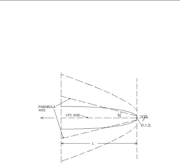
The parameters described are shown in Figure 2.16:

FIGURE 2.16 - Compound Parabolic Concentrator

The Origin is represented by the (X, Y, Z) coordinates, L is the Front length, θi is the angle Axis tilt, and ρ0 is the Lateral focal shift.

To make a textbook, or optimal CPC, you can pick the acceptance angle (equal to the axis tilt angle) and the exit port radius, then solve for the focal length and the overall length of the concentrator. The focal length f is found from

f = a(1 + sinθ1),

(2.3)

where a is the exit port radius and θi is the acceptance angle, and the overall length L is found from

	L =	a(1 + sinθ1)cosθ1	=	f cosθ1	,	(2.4)
		---------------------------------------------sin2θ1		---------------sin2θ1

2.18	TracePro 5.0 User’s Manual