2.7. FILTERING		67
	where a21 =³−³b11 + ´βb21 +	b12	+ b22´, a22 = 1 + r11 −βr21 + b22 +	b12	,
		β		β

and a23 = − b22 + bβ12 . Together you have the VAR(2)

"

zt

#

=

"

a21

a22

# "

zt−1

# +

" 0

a23

# "

zt−2

#

∆qt

a11

a12

∆qt−1

0

a13

∆qt−2

+

" uqt

uqt

# .

(2.98)

−

βuft

(2.98) is easier to estimate than the VECM and the standard forecasting formulae for VARs can be employed without modiÞcation.

2.7Filtering

Many international macroeconomic time-series contain a trend. The trend may be deterministic or stochastic (i.e., a unit root process). Real business cycle (RBC) theories are designed to study the cyclical features of the data, not the trends. So in RBC research, the data that is being studied is usually passed through a linear Þlter to remove the low-frequency or trend component of the data. To understand what Þltering does to the data you need to have some understanding of the frequency or spectral representation of time series where we think of the observations as being built up from individual subprocesses that exhibit cycles over di erent frequencies.

Linear Þlters take a possibly two-sided moving average of an original set of observations qt to create a new series q˜t

	∞
q˜t =		ajqt−j,		(2.99)
	=
	j X−∞
where the weights are summable,		∞	|aj| < ∞. One way to assess
		j=−∞
how the Þlter transforms the	properties of the original data is to see
		P

which frequency components from the original data that are allowed to pass through and how these frequency components are weighted—that is, are the particular frequency components that are allowed through relatively more or less important than they were in the original data.

68 CHAPTER 2. SOME USEFUL TIME-SERIES METHODS

The Spectral Representation of a Time Series

In section 2.4, a unit-root time series was decomposed into the sum of a random walk and a stationary AR(1) component. Here, we want to think of the time-series observations as being built up of underlying cyclical (cosine) functions each with di erent amplitudes and exhibiting cycles of di erent frequencies. A key question in spectral analysis is, which of these frequency components are relatively important in determining the behavior of the observed time-series?

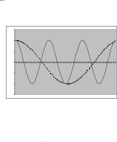
To Þx ideas, begin with the deterministic time-series, qt = a cos(ωt), where time is measured in years. This function exhibits a cycle every t = 2ωπ years. By choosing values of ω between 0 and π, you can get the process to exhibit cycles at any length that you desire. This is illustrated in Figure 2.1 where q1t = a cos(t) exhibits a cycle every 2π = 6.28 years and q2t = a cos(πt) displays a cycle every 2 years.

1.5
1
0.5
0
0	0.4	0.8	1.2	1.6	2	2.4	2.8	3.2	3.6	4	4.4	4.8	5.2	5.6	6
-0.5
-1
-1.5
Figure 2.1:	Deterministic Cycles—q1t							=	cos(t) (dashed) cycles every
2π = 6.28 years and q2t				= cos(πt) (solid) cycles every 2 years.

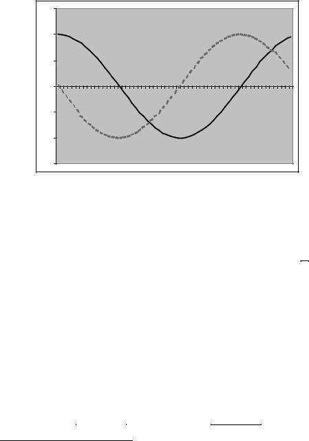
Something is clearly missing at this point and it is randomness. We introduce uncertainty with a random phase shift. If you compare q1t = a cos(t) to q3t = a cos(t + π/2), q3t is just q1t with a phase shift (horizontal movement) of π2 . This phase shift is illustrated in Figure 2.2

2.7. FILTERING																	69
˜			29		. Imagine that we take a draw from this distribu-
Now let λ U[0, π]
1.5
1
0.5
0
0	0.4	0.8		1.2		1.6	2	2.4	2.8	3.2	3.6	4	4.4	4.8	5.2	5.6	6
-0.5
-1
-1.5
Figure 2.2: π/2Phase shift. Solid: cos(t), Dashed: cos(t + π/2).

tion. Let the realization be λ, and form the time-series

qt = a cos(ωt + λ).

(2.100)

Once λ is realized, qt is a deterministic function with periodicity 2ωπ and phase shift λ but qt is a random function ex ante. We will need the following two basic trigonometric relations.

Two useful trigonometric relations. Let b and c be constants, and i be the imaginary number where i2 = −1. Then

cos(b + c)	=	cos(b) cos(c) − sin(b) sin(c)	(2.101)
eib	=	cos(b) + i sin(b)	(2.102)

(2.102) is known as de Moivre’s theorem. You can rearrange it to get

cos(b) =	(eib + e−ib)	, and	sin(b) =	(eib − e−ib)	.	(2.103)
	2
				2i

29You only need to worry about the interval [0, π] because the cosine function is symmetric about zero—cos(x) = cos(−x) for 0 ≤ x ≤ π

70 CHAPTER 2. SOME USEFUL TIME-SERIES METHODS

Now let b = ωt and c = λ and use (2.101) to represent (2.100) as

qt = a cos(ωt + λ)

= cos(ωt)[a cos(λ)] − sin(ωt)[a sin(λ)].

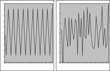
Next, build the time-series qt = q1t + q2t from the two sub-series q1t and q2t, where for j = 1, 2

qjt = cos(ωjt)[aj cos(λj)] − sin(ωjt)[aj sin(λj)],

and ω1 < ω2. The result is a periodic function which is displayed on the left side of Figure 2.3.

1								30
0.8								20
0.6
0.4								10
0.2
0								0
-0.2								-10
-0.4
-0.6								-20
-0.8
-1								-30
1	6	11	16	21	26	31	36	1	6	11	16	21	26	31	36

Figure 2.3: For 0 ≤ ω1 < · · · < ωN ≤ π, qt =		jN=1 qjt, where qjt =
cos(ωjt)[aj cos(λj)] − sin(ωjt)[aj sin(λj)]. Left	panel: N = 2. Right
		P

panel: N = 1000

The composite process with N = 2 is clearly deterministic but if you build up the analogous series with N = 100 of these components, as shown in the right panel of Figure 2.3, the series begins to look like a random process. It turns out that any stationary random process can be arbitrarily well approximated in this fashion letting N → ∞.

2.7. FILTERING

71

To summarize at this point, for su ciently large number N of these underlying periodic components, we can represent a time-series qt as

N
jX
qt = cos(ωjt)uj − sin(ωjt)vj,	(2.104)
=1

where uj = aj cos(λj) and vj = aj sin(λj), E(u2i ) = σi2, E(uiuj) = 0, i 6= j, E(vi2) = σi2, E(vivj) = 0, i 6= j.

Now suppose that E(uivj) = 0 for all i, j and let N → ∞.30 You are carving the interval into successively more subintervals and are cramming more ωj into the interval [0, π]. Since each uj and vj is associated with an ωj, in the limit, write u(ω) and v(ω) as functions of ω. For future reference, notice that because cos(−a) = cos(a), we

have u(−ω)

= u(ω) whereas because sin(−a) =

−sin(a), you have

v(−ω) = −v(ω). The limit of sums of the areas in these intervals is the

integral

qt = Z0π cos(ωt)du(ω) − sin(ωt)dv(ω).

(2.105)

Using (2.103), (2.105) can be represented as

t

Z0

2

− Z0

2i

q

=

π

eiωt + e−iωt

du(ω)

π

eiωt − e−iωt

dv(ω) .

(2.106)

|

}

({z

a)

Let dz(ω) =

1

[du(ω) + idv(ω)]. The second integral labeled (a) can be

simpliÞed as

2

(49)

Z0		2i		Z0	2i
	π	eiωt − e−iωt	dv(ω) =	π	eiωt − e−iωt
				Z0π	e−iωt − eiωt
	=
					2
	=			Z0π(e−iωt − eiωt

Ã!

2dz(ω) − du(ω) i

(2dz(ω) − du(ω))

Z π eiωt − e−iωt

)dz(ω) + du(ω).

0 2

Substitute this last result back into (2.106) and cancel terms to get

(50)

30This is in fact not true because E(uivi) =6 0, but as we let N → ∞, the importance of these terms become negligible.

72 CHAPTER 2. SOME USEFUL TIME-SERIES METHODS

qt

= Z0π e−iωtdu(ω) + Z0π eiωtdz(ω) −Z0π e−iωtdz(ω) .

(2.107)

|

{z

} |

({zb)

} |

({z

}

(a)

c)

π

−

0

Since u( ω) = u(ω), the term labeled (a) in (2.107) can be written as

R0

e−iωtdz(ω) =

R2

0 e−iωtdu(ω) +

2

0

ie−iωtdv(ω) =

2

π eiωtdu(ω)

0

e−iωtdu(ω) =

−π eiωtdu(ω). The third term labeled (c) in (2.107) is

R

π

π ie dv(ω).

1

R

π

1

R

π

1

R

0

−

(51)

1

R

0

π

iωt

t

=

2

−π e

−

0

iωt

[du(ω) + idv(ω)] +

e dz(ω)

2

−

Substituting these results back into (2.107) and can-

celing

terms

you

get,

q

1

0

iωt

π

iωt

=

R

known as the Cramer Representation of q ,

−π e

dz(ω).

This is

R

R

t

which we restate as

N

−

X

lim

π

iωtdz(ω).

(2.108)

qt = N→∞ j=1 aj cos(ωjt + λj) = Z

π e

The point of all this is that any time-series can be thought of as be-

ing built up from a set of underlying subprocesses whose individual

frequency components exhibit cycles of varying frequency. The other

side of this argument is that you can, in principle, take any time-series

qt and Þgure out what fraction of its variance is generated from those

subprocesses that cycle within a given frequency range. The business

cycle frequency, which lies between 6 and 32 quarters is of key interest

to, of all people, business cycle researchers.

Notice that the process dz(ω) is built up from independent incre-

ments. For coincident increments, you can deÞne the function s(ω)dω

to be

s(ω)dω

λ = ω

E[dz(ω)dz(λ)] = (

,

(2.109)

0

otherwise

where

an

overbar

denotes

the

complex conjugate.31

Since

eiωt

eiωt

= cos2(ωt) + sin2(ωt) =

1 at frequency ω, it follows that

E[eiωt

eiωt

dz(ω)dz(ω)] = s(ω)dω.

That is, s(ω)dω is the variance of

the ω−frequency component of qt, and is called the spectral density

function of qt. Since by (2.108), qt is built up from frequency compo-

nents ranging from [−π, π], the total variance of qt must be the integral

31If a and b are real numbers and z = a + bi is a complex number, the complex conjugate of z is z¯ = a − bi. The product zz¯ = a2 + b2 is real.

2.7. FILTERING		73
of s(ω). That is32
	π			π
E(qt2) = E[Z−π eiωtdz(ω) Z−π
					eiλtdz(λ)]
= E[Z	π	Z π eiωt		dz(ω)
			eiλt			dz(λ)]

Zπ −π −π

=E[dz(ω)dz(λ)]

Z−ππ

=

s(ω)dω.

(2.110)

−π

The spectral density and autocovariance generating functions. The autocovariance generating function for a time series qt is deÞned to be

	∞
g(z) =	γjzj,
	=
	j X−∞

where γj = E(qtqt−j) is the j-th autocovariance of qt. If we let z = e−iω,

then

2π Z

π g(e−iω)eiωkdω =

2π j=

γj Z

π eiω(k−j)dω.

1

π

1

∞

π

−

X−∞

−

Let a = k

−

j. Then eiωa = cos(ωa)+i sin(ωa) and the integral becomes,

R

π

R

π

−

π

π

−π cos(ωa)dω +i

−π sin(ωa)dω = (1/a) sin(aω)|−π −(i/a) cos(aω)|−π.

The second term is 0 because cos(

aπ) = cos(aπ).

The Þrst term

is 0 too because the sine of any nonzero integer multiple of π is 0 and a is an integer. Therefore, the only value of a that matters is

a = k

−

j = 0, which implies that γ

=

1

π g(e−iω)eiωkdω. Setting

1

kπ

2π

−π

t) =

−π s(ω)dω, so the

R

k = 0, you have γ0 = Var(qt) = 2π

π g(e−Riω)dω, but you know that

Var(q

π

−

spectral density function is proportional

to the

autocovariance generating function with z = e iω. Notice also,

R

∞

−

that when you set ω = 0, then s(0) =

γj. The spectral density

j=−∞

function of qt at frequency 0 is the

same thing as the long-run variance

P

of qt. It follows that

2π Z−π g(e−iω)dω,

(2.111)

Var(qt) = Z−π s(ω)dω =

π

1

π

where g(z) = P∞ γjzj.

j=−∞

32We obtain the last equality because dz(ω) is a process with independent increments so unless λ = ω, Edz(ω)dz(λ) = 0.

(52)

(53)