6.1. DEVIATIONS FROM UIP

167

Hansen-Hodrick t-ratios tHH are given in square brackets and OLS t- ratios tOLS are given in double parentheses. The relative range is the 2.5 to 97.5 percentile of the distribution with overlapping observations divided by the 2.5 to 97.5 percentile of the distribution with nonoverlapping observations.2 The empirical distribution of each statistic is based on 2000 replications.

You can see that there deÞnitely is an e ciency gain to using overlapping observations. The range encompassing the 2.5 to 97.5 percentiles of the Monte Carlo distribution of the OLS estimator shrinks approximately by half when going from nonoverlapping (quarterly) to overlapping (monthly) observations. The tradeo is that for very small samples, the distribution of the t-ratios under overlapping observations are more fat-tailed and look less like the standard normal distribution than the OLS t-ratios.

Fama Decomposition Regressions

Although the preceding Monte Carlo experiment suggested that you can achieve e ciency gains by using overlapping observations, in the interests of simplicity, we will go back to working with the log oneperiod forward rate, ft = ft,1 to avoid inducing the moving average errors.

DeÞne the expected excess nominal forward foreign exchange payo to be

pt ≡ ft − Et[st+1],

(6.1)

where Et[st+1] = E[st+1|It]. You already know from the Hansen—Hodrick regressions that pt is non zero and that it evolves overtime as a random process. Adding and subtracting st from both sides of (6.1) gives

ft − st = Et(st+1 − st) + pt.

(6.2)

Fama [48] shows how to deduce some properties of pt using the analysis of omitted variables bias in regression problems. First, consider the regression of the ex post forward proÞt ft − st+1 on the current period forward premium ft −st. Second, consider the regression of the

2For example, we get the row 1 relative range value 0.471 for the slope coe cient from (1.207-0.778)/(1.453-0.543).

168CHAPTER 6. FOREIGN EXCHANGE MARKET EFFICIENCY

one-period ahead depreciation st+1 − st on the current period forward premium. The regressions are

ft − st+1	=	α1 + β1(ft − st) + ε1t+1,	(6.3)
st+1 − st	=	α2 + β2(ft − st) + ε2t+1.	(6.4)

(6.3) and (6.4) are not independent because when you add them together you get

α1 + α2	=	0,
β1 + β2	=	1,	(6.5)
ε1t+1 + ε2t+1	=	0.	(6.6)

In addition, these regressions have no structural interpretation. So why was Fama interested in running them? Because it allowed him to estimate moments and functions of moments that characterize the joint distribution of pt and Et(st+1 − st).

The population value of the slope coe cient in the Þrst regression (6.3) is β1 = Cov[(ft − st+1), (ft − st)]/Var[ft − st]. Using the deÞnition of pt, it follows that the forward premium can be expressed as, ft − st = pt + E(∆st+1|It) whose variance is Var(ft − st) = Var(pt) + Var[E(∆st+1|It)]+2Cov[pt, E(∆st+1|It)]. Now add and subtract E(st+1|It) to the realized proÞt to get ft − st+1 = pt − ut+1 where ut+1 = st+1 − E(st+1|It) = ∆st+1 − E(∆st+1|It) is the unexpected depreciation. Now you have, Cov[(ft −st+1), (ft −st)] = Cov[(pt −ut+1), (pt +E(∆st+1|It))] = Var(pt) + Cov[pt, E(∆st+1|It))]. With the aid of these calculations, the slope coe cient from the Þrst regression can be expressed as

β1 =	Var(pt) + Cov[pt, Et(∆st+1)]
	Var(pt) + Var[Et(∆st+1)] + 2Cov[pt, Et(∆st+1)].	(6.7)

In the second regression cient is β2 = Cov[(∆st+1 substitutions yields

(6.4), the population value of the slope coe - ), (ft −st)]/Var(ft −st). Making the analogous

β2 =	Var[Et(∆st+1)] + Cov[pt, Et(∆st+1)]
	Var(pt) + Var[Et(∆st+1)] + 2Cov[pt, Et(∆st+1)].	(6.8)

6.1. DEVIATIONS FROM UIP							169
	Table 6.3: Estimates of Regression Equations (6.3) and (6.4)
		US-BP	US-JY	US-DM	DM-BP	DM-JY	BP-JY
	ˆ	-3.481	-4.246	-0.796	-1.645	-2.731	-4.295
	β2
	t(β2 = 0)	(-2.413)	(-3.635)	(-0.542)	(-1.326)	(-1.797)	(-2.626)
	t(β2 = 1)	(-3.107)	(-4.491)	(-1.222)	(-2.132)	(-2.455)	(-3.237)
	ˆ	4.481	5.246	1.796	2.645	3.731	5.295
	β1
Notes: Nonoverlapping quarterly observations from 1976.1 to 1999.4.							t(β2 = 0)
(t(β2 = 1) is the t-statistic to test β2 = 0 (β2 = 1).

Let’s run the Fama regressions using non-overlapping quarterly observations from 1976.1 to 1999.4 for the British pound (BP), yen (JY), deutschemark (DM) and dollar (US). We get the following results.

There is ample evidence that the forward premium contains useful information for predicting the future depreciation in the (generally) sig-

ˆ

niÞcant estimates of β2. Since β2 is signiÞcantly less than 1, uncovered interest parity is rejected. The anomalous result is not that β2 6= 1, but that it is negative. The forward premium evidently predicts the future depreciation but with the “wrong” sign from the UIP perspective. Recall that the calibrated Lucas model in chapter 4 also predicts a negative β2 for the dollar-deutschemark rate.

The anomaly is driven by the dynamics in pt. We have evidence that it is statistically signiÞcant. The next question that Fama asks is whether pt is economically signiÞcant. Is it big enough to be economically interesting? To answer this question, we use the estimates and the slope-coe cient decompositions (6.7) and (6.8) to get information

about the relative volatility of pt.
	ˆ	< 0. From (6.8) it follow that pt			must be nega-
First note that β2
tively	correlated	with	the	expected	depreciation,

Cov[pt, E(∆st+1|It)] < 0. By (6.5), the negative estimate of β2 implies

ˆ	> 0. By (6.7), it must be the case that Var(pt) is large enough
that β1
	ˆ	ˆ	> 0, it follows
to o set the negative Cov(pt, Et(∆st+1)). Since β1		− β2

that Var(pt) > Var(E(∆st+1|It)), which at least places a lower bound on the size of pt.

170CHAPTER 6. FOREIGN EXCHANGE MARKET EFFICIENCY

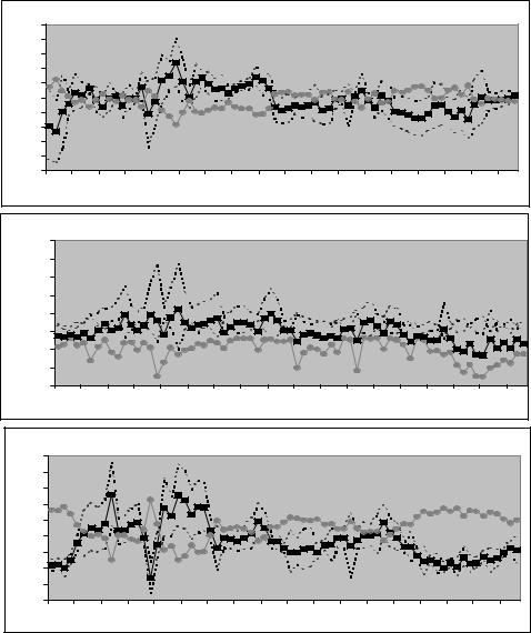
Estimating pt

We have evidence that pt = ft − E(st+1|It) evolves as a random process, but what does it look like? You can get a quick estimate of pt by projecting the realized proÞt ft − st+1 = pt − ut+1 on a vector of observations zt where ut+1 = st+1 −E(st+1|It) is the rational prediction error. Using the law of iterated expectations and the property that

E(ut+1|zt) = 0, you have E(ft − st+1|zt) = E(pt|zt). If you run the regression

ft − st+1 = zt0β + ut+1,

you can use the Þtted value of the regression as an estimate of the ex

ante payo , pˆt = zt0 βˆ.

A slightly more sophisticated estimate can be obtained from a vector

error correction representation that incorporates the joint dynamics of

the spot and forward rates. Here, the log spot and forward rates are as-

sumed to be unit root processes and the forward premium is assumed to

be stationary. The spot and forward rates are cointegrated with cointe-

gration vector (1, −1). As shown in chapter 2.6, st and ft have a vector

error correction representation which can be represented equivalently

as a bivariate vector autoregression in the forward premium (ft − st)

and the depreciation ∆st.

Let’s pursue the VAR option. Let

y

t = (ft − st, ∆st)0 follow the

k−th order VAR

k

jX

y

t

=

Ajy

t−j

+ vt.

=1

(109)

Let e2 = (0, 1) be a selection vector such that e2

y

t = ∆st picks o the

depreciation, and Ht = (y

, y

t−1

, . . .) be current and lagged values of

t

P

y

t. Then E(∆st+1|Ht) = e2E(

y

t+1|Ht) = e2 h

jk=1 Aj

y

t+1−ji, and you

6.1. DEVIATIONS FROM UIP

171

A. US-UK

50
40
30
20
10
0
-10
-20
-30
-40
-50
1976	1978	1980	1982	1984	1986	1988	1990	1992

B. US-Germany

50
40
30
20
10
0
-10
-20
-30
1976	1978	1980	1982	1984	1986	1988	1990	1992

C. US-Japan

50
40
30
20
10
0
-10
-20
-30
-40
1976	1978	1980	1982	1984	1986	1988	1990	1992

Figure 6.1: Time series point estimates of pt (boxes) with 2-standard error bands and point estimates of Et(∆st+1) (circles).