8.4. VAR ANALYSIS OF MUNDELL—FLEMING

257

Appendix: Solving the Dornbusch Model

From (8.9) and (8.11), we see that the behavior of i(t) is completely determined by that of s(t). This means that we need only determine the di erential equations governing the exchange rate and the price level to obtain a complete characterization of the system’s dynamics.

Substitute (8.9) and (8.11) into (8.6). Make use of (8.13) and rearrange

to obtain		1
				[p(t) − p¯].				(8.58)
	sú(t) =
			λ
To obtain the di erential equation for the price level, begin by substituting
(8.58) into (8.9), and then substituting the result into (8.8) to get								(144)
pú(t) = π[δ(s(t) − p(t)) + (γ − 1)y − σi −						σ
							(p(t) − p¯) + g].	(8.59)
						λ
However, in the long run
	0 = π[δ(¯s − p¯) + (γ − 1)y − σr + g],							(8.60)
the price dynamics are more conveniently characterized by								(145)
	pú(t) = π ·δ(s(t) − s¯) − (δ + λ )(p(t) − p¯)¸ ,							(8.61)
					σ
which is obtained by subtracting (8.60) from (8.59).
Now write (8.58) and (8.61) as the system
	Ã pú(t)	! = A Ã p(t) − p¯ ! ,						(8.62)
	sú(t)			s(t) s¯
					−
where	Ã	!

01/λ

A =	πδ	−π(δ + σ/λ)	.

(8.62) is a system of two linear homogeneous di erential equations. We know that the solutions to these systems take the form

s(t)	=	s¯ + αeθt,	(8.63)
p(t)	=	p¯ + βeθt.	(8.64)

We will next substitute (8.63) and (8.64) into (8.62) and solve for the unknown coe cients, α, β, and θ. First, taking time derivatives of (8.63)

and (8.64) yields
sú	=	θαeθt,	(8.65)
pú	=	θβeθt.	(8.66)

	258	CHAPTER 8. THE MUNDELL-FLEMING MODEL
	Substitution of (8.65) and (8.66) into (8.62) yields
						(A − θI2) Ã β			! = 0.		(8.67)
								α
	In order for (8.67) to have a solution other than the trivial one (α, β) = (0, 0),
	requires that
				0 =			|A − θI2|				(8.68)
				=			θ2 − T r(A)θ + |A|,				(8.69)
(146)	where Tr(A) = −π(δ + σ/λ) and |A| = −πδ/λ otherwise, (A −θI2)−1 exists
	which means that the unique solution is the trivial one, which isn’t very
	interesting. Imposing the restriction that (8.69) is true, we Þnd that its
	roots are	θ1	=		2[T r(A) − qT r2(A) − 4|A|] < 0,						(8.70)
					1
		θ2	=		2[T r(A) + qT r2(A) − 4|A|] > 0.						(8.71)
	The general solution is			1
				s(t) =			s¯ + α1eθ1t + α2eθ2t,				(8.72)
				p(t) =			p¯ + β1eθ1t + β2eθ2t.				(8.73)

This solution is explosive, however, because of the eventual dominance of the positive root. We can view an explosive solution as a bubble, in which the exchange rate and the price level diverges from values of the economic fundamentals. While there are no restrictions within the model to rule out explosive solutions, we will simply assume that the economy follows the stable solution by setting α2 = β2 = 0, and study the solution with the stable root

θ ≡ −θ1										(8.74)
= 2[π(δ + σ/λ) + qπ2(δ + σ/λ)2 + 4πδ/λ].										(8.75)
1
Now, to Þnd the stable solution, we solve (8.67) with the stable root
0 = (A − θ1I2)				Ã β		!
Ã					α			β !
		πδ		θ1		π(δ + σ/λ) ! Ã
=		−θ1	−		−	1/λ		α .
										(8.76)

8.4. VAR ANALYSIS OF MUNDELL—FLEMING						259
When this is multiplied out, you get
0	=	−θ1α + β/λ,	µδ + λ		¶]β.	(8.77)
0	=	πδα − [θ1 + π				(8.78)
				σ
It follows that
		α = β/θ1λ.				(8.79)

Because α is proportional to β, we need to impose a normalization. Let this normalization be β = po − p¯ where po ≡ p(0). Then α = (po − p¯)/θ1λ = −[po − p¯]/θλ, where θ ≡ −θ1. Using these values of α and β in (8.63) and (8.64), yields

p(t)	=	p¯ + [po − p¯]e−θt,	(8.80)
s(t)	=	s¯ + [so − s¯]e−θt,	(8.81)

where (so − s¯) = −[po − p¯]/θλ. This solution gives the time paths for the price level and the exchange rate.

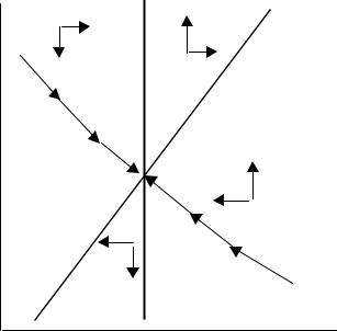
To characterize the system and its response to monetary shocks, we will want to phase diagram the system. Going back to (8.58) and (8.61), we see that sú(t) = 0 if and only if p(t) = p¯, while pú(t) = 0 if and only if s(t) −s¯ = (1+ σ/λδ)(p(t) −p¯). These points are plotted in Figure 8.10. The system displays a saddle path solution.

260	CHAPTER 8. THE MUNDELL-FLEMING MODEL

s	.

p=0

.

s=0

p

Figure 8.10: Phase diagram for the Dornbusch model.