3.5. TESTING MONETARY MODEL PREDICTIONS

91

where we have used the fact that γ = 1 − ψ. Some additional algebra reveals

Var(∆st) =	(1 − ρψ)2 + 2ρψ(1 − ρ)	Var(∆ft) > Var(∆ft).
	(1 − ρψ)2

This is not very encouraging since the levels of the fundamentals are explosive. The end-of-chapter problems show that neither an AR(1) nor a permanent—transitory components representation (chapter 2.4) for the fundamentals allows the monetary model to explain why exchange rate returns are more volatile than the growth rate of the fundamentals.

3.5Testing Monetary Model Predictions

This section looks at two empirical strategies for evaluating the monetary model of exchange rates.

MacDonald and Taylor’s Test

The Þrst strategy that we look at is based on MacDonald and Taylor’s [96] adaptation of Campbell and Shiller’s [20] tests of the present value model.3 This section draws on material on cointegration presented in chapter 2.6.

Let It be the time t information set available to market participants. Subtracting ft from both sides of (3.8) gives

st − ft = λE(st+1 − st|It) = λ(it − it ).

(3.17)

st is by all indications a unit-root process, whereas ∆st and E(∆st+1|It) are clearly stationary. It follows from the Þrst equality in (3.17) that st and ft must be cointegrated. Using (3.12) and noting that ψ = λγ gives

λEt(∆st+1) = λ	γ	∞	ψjEtft+1+j − γ	∞	ψjEtft+j
		jX		X
		=0		j=0

3The seminal contributions to this literature are Leroy and Porter [90] and Shiller [127].

92	CHAPTER 3. THE MONETARY MODEL
	∞
	jX
=	ψjEt∆ft+j.	(3.18)
	=1

(3.17) and (3.18) allow you to represent the deviation of the exchange rate from the fundamental as the present value of future fundamentals growth

∞
jX
ζt = st − ft = ψjEt∆ft+j.	(3.19)
=1

Since st and ft are cointegrated they can be represented by a vector error correction model (VECM) that describes the evolution of (∆st, ∆ft, ζt), where ζt ≡ st − ft. As shown in chapter 2.6, the linear dependence among (∆st, ∆ft, ζt) induced by cointegration implies that the information contained in the VECM is preserved in a bivariate vector autoregression (VAR) that consists of ζt and either ∆st or ∆ft. Thus we will drop ∆st and work with the p−th order VAR for (∆ft, ζt)

		p					−
	∆ft	jX	a11,j	a12,j					²t
Ã	ζt	! =	Ã a21,j	a22,j	! Ã	ζt	−j	!	+ Ã vt	! .	(3.20)
		=1

The information set available to the econometrician consists of current and lagged values of ∆ft and ζt. We will call this information Ht = {∆ft, ∆ft−1, . . . , ζt, ζt−1, . . .}. Presumably Ht is a subset of economic agent’s information set, It. Take expectations on both sides of (3.19) conditional on Ht and use the law of iterated expectations to get4

∞
jX
ζt = ψjE(∆ft+j|Ht).	(3.21)
=1

What is the point of deriving (3.21)? The point is to show that you can use the prediction formulae implied the data-generating process (3.20) to compute the necessary expectations. Expectations of market participants E(∆ft+j|It) are unobservable but you can still test the theory by substituting the true expectations with your estimate of these expectations, E(∆ft+j|Ht).

4Let X, Y, and Z be random variables. The law of iterated expectations says E[E(X|Y, Z)|Y ] = E(X|Y ).

3.5. TESTING MONETARY MODEL PREDICTIONS

93

To simplify computations of the conditional expectations of future fundamentals growth, reformulate the VAR in (3.20) in the VAR(1) companion form

where
		Y t =
		1	0
		a11,1	a11,2
		0	1
	..
	.		· · ·
		0
			· · ·
B =
		0
			· · ·
	a21,1		a21,2
		0
			· · ·
	..
	.		· · ·
		0
			· · ·

Y t = BY t−1 + ut,

∆ft		t 1					0t
∆f							²
	..					..
	. −						.
∆ft p+1				,	ut =		0
−								,
ζt						vt
ζt		1					0
	−
	..					..
	.					.
ζt p+1							0
−
· · ·			a11,p		a12,1 a12,2			· · ·
· · ·			0		0	0		· · ·
0 · · ·			0		0	0		· · ·
			.		.	.		.
			.		.	.		.
· · · .					.	.		.
· · · 1			0		0	· · ·		· · ·
· · ·			a21,p		a22,1 a22,2			· · ·
· · ·			0		1	0		· · ·
· · ·			0		0	1		0 · · ·
			.		.	.		.
			.		.	.		.
· · · .					.	.		.
· · ·			0		0	· · ·		· · · 1

(3.22)

0
a12,p
0
..
.
0
a22,p
0
0
..
.
0

Now let e1 be a (1 × 2p) row vector with a 1 in the Þrst element and zeros elsewhere and let e2 be a (1 × 2p) row vector with a 1 as the p + 1−th element and zeros elsewhere

e1 = (1, 0, . . . , 0), e2 = (0, . . . , 0, 1, 0, . . . , 0).
These are selection vectors that give	(65)
e1Y t = ∆ft, e2Y t = ζt.
Now the k-step ahead forecast of ft is conveniently expressed as
E(∆ft+j|Ht) = e1E(Y t+j|Ht) = e1BjY t.	(3.23)

94		CHAPTER 3. THE MONETARY MODEL
Substitute (3.23) into (3.21) to get
				∞
				jX
ζ	= e Y	t	= ψje BjY				t
t	2					1
				=1
					jX
			=	e1		∞ ψjBj Yt		(3.24)
						=1

= e1ψB(I − ψB)−1Y t.

Equating coe cients on elements of Y t yields a set of nontrivial restrictions predicted by the theory which can be subjected to statistical hypothesis tests

e2(I − ψB) = e1ψB.

(3.25)

Estimating and Testing the Present-Value Model

We use quarterly US and German observations on the exchange rate, money supplies and industrial production indices from the International Financial Statistics CD-ROM from 1973.1 to 1997.4, to re-estimate the MacDonald and Taylor formulation and test the restrictions (3.25). We view the US as the home country. The bivariate VAR is run on (∆ft, ζt) with observations demeaned prior to estimation. The fundamentals are given by ft = (mt −mt )−(yt −yt ) where the income elasticity of money demand is Þxed at φ = 1.

The BIC (chapter 2.1) tells us that a VAR(4) is the appropriate. Estimation proceeds by letting x0t = (∆ft−1, . . . , ∆ft−4, ζt−1, . . . , ζt−4) and running least squares on

∆ft = x0tβ + ²t,

ζt = x0tδ + vt.

Expanding (3.25) and making the correspondence between the co- e cients in the matrix B and the regressions, we write out the testable restrictions explicitly as

β1 + δ1 = 0,	β5 + δ5 = 1/ψ,
β2 + δ2 = 0,	β6 + δ6 = 0,
β3 + δ3 = 0,	β7 + δ7 = 0,
β4 + δ4 = 0,	β8 + δ8 = 0.

3.5. TESTING MONETARY MODEL PREDICTIONS

95

These restrictions are tested for a given value of the interest semielasticity of money demand, λ = ψ/(1 − ψ). To set up the Wald test,

let π0 = (β0, δ0) be the grand coe cient vector from the OLS regressions, (70)

R = (I8 : I8) be the restriction matrix and r0 = (0, 0, 0, 0, (1/ψ), 0, 0, 0),

ΩT

= ΣT

Q−1, where ΣT

=

1

²

²0, QT =

1

x

x0 . Then as

→ ∞

T

t

t

T

P

P

, the Wald statistic

T

t

T

t

W = (Rπ − r)0

D

[RΩT R0]−1(Rπ − r) χ82.

Here are the results. The Wald statistics and their associated values of λ are W = 284, 160(λ = 0.02), W = 113, 872(λ = 0.10), W = 44, 584(λ = 0.16), and W = 18, 291(λ = 0.25). The restrictions are strongly rejected for reasonable values of λ.

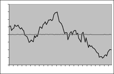
One reason why the model fares poorly can be seen by comparing the theoretically implied deviation of the spot rate from the fundamentals

˜	ψB(I − ψB)	−1	Yt,
ζt = e1

which is referred to as the ‘spread’ with the actual deviation, ζt = st−ft. These are displayed in Figure 3.5 where you can see that the implied spread is much too smooth.

Long-Run Evidence for the Monetary Model from Panel Data

The statistical evidence against the rational expectations monetary model is pretty strong. One of the potential weak points of the model is that PPP is assumed to hold as an exact relationship when it is probably more realistic to think that it holds in the long run.

Mark and Sul [101] investigate the empirical link between the monetary model fundamentals and the exchange rate using quarterly observations for 19 industrialized countries from 1973.1 to 1997.4 and the

panel exchange rate predictive regression		(72)
sit+k − sit = βζit + ηit+k,	(3.26)
where ηit+k = γi + θt+k + uit+k has an error-components representa-		(73)
tion with individual e ect γi, common time e ect θt and idiosyncratic

96	CHAPTER 3. THE MONETARY MODEL

Table 3.2: Monetary fundamentals out-of-sample forecasts of US dollar returns with nonparametric bootstrapped p-values under cointegration.

		1-quarter ahead			16-quarters ahead
	Country	U-statistic p-value			U-statistic p-value
	Australia	1.024	0.904		0.864	0.222
	Austria	0.984	0.013		0.837	0.131
	Belgium	0.999	0.424		0.405	0.001
	Canada	0.985	0.074		0.552	0.009
	Denmark	1.014	0.912		0.858	0.174
	Finland	1.001	0.527		0.859	0.164
	France	0.994	0.155		0.583	0.004
	Germany	0.986	0.056		0.518	0.003
	Great Britain	0.983	0.077		0.570	0.012
	Greece	1.016	0.909		1.046	0.594
	Italy	0.997	0.269		0.745	0.016
	Japan	1.003	0.579		0.996	0.433
	Korea	0.912	0.002		0.486	0.012
	Netherlands	0.986	0.041		0.703	0.032
	Norway	0.998	0.380		0.537	0.002
	Spain	0.996	0.341		0.672	0.028
	Sweden	0.975	0.034		0.372	0.001
	Switzerland	0.982	0.008		0.751	0.049
	Mean	0.991	0.010		0.686	0.001
	Median	0.995	0.163		0.688	0.001

Notes: Bold face indicate statistical signiÞcance at the 10 percent level.

3.5. TESTING MONETARY MODEL PREDICTIONS

97

e ect uit+k. A panel combines the time-series observations of several cross-sectional units. The individuals in the cross section are di erent countries which are indexed by i = 1, . . . , N.

Out-of-Sample Fit and Prediction

Mark and Sul’s primary objective is to use the regression to generate out-of-sample forecasts of the depreciation. They base their methodology on the work of Meese and Rogo [104] who sought to evaluate the empirical performance of alternative exchange rate models that were popular in the 1970s by conducting a monthly postsample Þt analysis.

Suppose there are j = 1, . . . J models under consideration. Let xjt (74) be a vector of exchange rate determinants implied by ‘model j,’ and

0j	β	j	j	be regression representation of model j. What Meese
st = xt			+ et

and Rogo did was to divide the complete size T (time-series) sample in two. Sample 1 consists of observations t = 1, . . . t1 and sample 2 consists of observations t = t1 + 1, . . . , T , where t1 < T . Using sample 1 to estimate βj, they then formed the out-of-estimation sample Þt of

		j	0j ˆ		for t = t1 + 1, . . . T .
the exchange rate predicted by model j sˆt			= xt β	j

The Meese—Rogo regressions were contemporaneous relationships between the dependent variable and the vector of independent variables. To truly generate forecasts of future values of st they needed to forecast future values of the xjt vectors. Instead, Meese and Rogo used realized values of the xjt vectors–hence the term out-of-sample Þt. The various models were judged on the accuracy of their out-of estimation sample Þt.

The models were compared to the predictions of the driftless random walk model for the exchange rate. This is an important benchmark for evaluation because the random walk says there is no information that helps to predict future change. You would think that an econometric model with any amount of economic content would dominate the ‘nochange’ prediction of the random walk. Even though they biased the results in favor of the model-based regressions by using realized values of the independent variables, Meese and Rogo found that that the out-of-sample Þt from the theory-based regressions were uniformly less accurate than the random walk.

Their study showed that many models may Þt well in sample but

98	CHAPTER 3. THE MONETARY MODEL

they have a tendency to fall apart out of sample. There are many possible explanations for the instability, but ultimately, the reason boils down to the failure to Þnd a time-invariant relationship between the exchange rate and the fundamentals. Although their conclusions regarding the importance of macroeconomic fundamentals for the exchange rate were nihilistic, Meese and Rogo established a rigorous tradition in international macroeconomics of using out-of-sample Þt or forecasting performance as model evaluation criteria.

Panel Long-Horizon Regression

Let’s return to Mark and Sul’s analysis. They evaluate the predictive content of the monetary model fundamentals by initially estimating the regression on observations through 1983.1. Note that the regressand in (3.26) are past (not contemporaneous) deviations of the exchange rate from the fundamentals. It is a predictive regression that generates actual out-of-sample forecasts. The k = 1 regression is used to forecast 1- quarter ahead, and the k = 16 regression is used to forecast 16 quarters ahead. The sample is then updated by one observation and a new set of forecasts are generated. This recursive updating of the sample and forecast generation is repeated until the end of the data set is reached. β = 0 if the monetary fundamentals contain no predictive content or if the exchange rate and the fundamentals do not cointegrate.

Let observations T − T0 to T be sample reserved for forecast evaluation. If sˆit+k −sit is the k−step ahead regression forecast formed at t, the root-mean-square prediction error (RMSPE) of the regression is

	= v
R1			1 T		(ˆsit	−	sit k)2.
	uT0			=T			−
	u			tX0
	t

The monetary fundamentals regression is compared to the random walk

iid 2

with drift, sit+1 = µi + sit + ²it where ²it (0, σi ). The k−step ahead forecasted change from the random walk is sˆit+k −sit = kµi. Let R2 be the random walk model’s RMSPE. Theil’s [134] statistic U = R1/R2 is the ratio of the RMSPE of the two models. The regression outperforms the random walk in prediction accuracy when U < 1.

Table 3.2 shows the results of the prediction exercise. The nonparametric residual bootstrap (see chapter 2.5) is used to generate p-values

3.5. TESTING MONETARY MODEL PREDICTIONS

99

for a test of the hypothesis that the regression and the random walk models give equally accurate predictions. There is a preponderance of statistically superior predictive performance by the monetary model exchange rate regression.

100	CHAPTER 3. THE MONETARY MODEL

20			Stock Returns andLog Dividend Yield										20					Dollar/Pound
15													15
10													10
5													5
													0
0
													-5
-5													-10
-10													-15
-15													-20
73	75	77	79	81	83	85	87	89	91	93	95	97	73	75	77	79	81	83	85	87	89	91	93	95	97
				Dollar/Deutschemark														Dollar/Yen

20													20
15													15
10													10
5													5
0													0
-5													-5
-10													-10
-15													-15
-20													-20
73	75	77	79	81	83	85	87	89	91	93	95	97	73	75	77	79	81	83	85	87	89	91	93	95	97

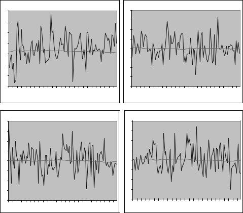
Figure 3.4: Quarterly stock and exchange rate returns (jagged line), 1973.1 through 1997.4, with price deviations from the fundamentals (smooth line).

3.5. TESTING MONETARY MODEL PREDICTIONS

101

0.8
0.6
0.4						Actual
0.2										Theoretical
0
-0.2
-0.4
-0.6
-0.8
74	76	78	80	82	84	86	88	90	92	94	96
Figure 3.5: Theoretical and actual spread, st − ft.

102	CHAPTER 3. THE MONETARY MODEL

Monetary Model Summary

1.The monetary model builds on purchasing-power parity, uncovered interest parity, and stable transactions-based money demand functions.

2.Domestic and foreign money and real income levels are the fundamental determinants of the nominal exchange rate.

3.The exchange rate is viewed as the relative price of two monies, which are assets. Since asset prices are in general more volatile than their fundamentals, it comes as no surprise that exchange rates exhibit excess volatility. The present value form of the solution underscores the concept that the exchange rate is an asset price.

4.The monetary model is a useful Þrst approximation in Þxing our intuition about exchange rate dynamics even though it fails to explain the data on many dimensions. Because purchasing power parity is assumed to hold as an exact relationship, the model cannot explain the dynamics of the real exchange rate. Indeed, the main reason to study nominal exchange rate behavior is if we think that nominal exchange rate movements are correlated with real exchange rate changes so that they have real consequences.