162CHAPTER 6. FOREIGN EXCHANGE MARKET EFFICIENCY

the data. The ensuing challenge is then to understand why uncovered interest parity fails.

We cover three possible explanations. The Þrst is that the forward foreign exchange rate contains a risk premium. This argument is developed using the Lucas model of chapter 4. The second explanation is that the true underlying structure of the economy is subject to change occasionally but economic agents only learn about these structural changes over time. During this transitional learning period in which market participants have an incomplete understanding of the economy and make systematic prediction errors even though they are behaving rationally. This is called the ‘peso-problem’ approach. The third explanation is that some market participants are actually irrational in the sense that they believe that the value of an asset depends on extraneous information in addition to the economic fundamentals. The individuals who take actions based on these pseudo signals are called ‘noise’ traders.

The notational convention followed in this chapter is to let upper case letters denote variables in levels and lower case letters denote their logarithms, with the exception of interest rates, which are always denoted in lower case. As usual, stars are used to denote foreign country variables.

6.1Deviations From UIP

Let s be the log spot exchange rate, f be the log one-period forward rate, i be the one-period nominal interest rate on a domestic currency (dollar) asset and i is the nominal interest rate on the foreign currency (euro) asset. If uncovered interest parity holds, it − it = Et(st+1) − st, but by covered interest parity, it −it = ft −st. Therefore, unbiasedness of the forward exchange rate as a predictor of the future spot rate ft = Et(st+1) is equivalent to uncovered interest parity.

We begin by covering the basic econometric analyses used to detect these deviations.

6.1. DEVIATIONS FROM UIP

163

Hansen and Hodrick’s Tests of UIP

Hansen and Hodrick [71] use generalized method of moments (GMM) to test uncovered interest parity. The GMM method is covered in chapter 2.2. The Hansen—Hodrick problem is that a moving-average serial correlation is induced into the regression error when the prediction horizon exceeds the sampling interval of the data.

The Hansen—Hodrick Problem

To see how the problem arises, let ft,3 be the log 3-month forward ex-

change rate at time t, st be the log spot rate, It be the time t information (102) set available to market participants, and Jt be the time t information

set available to you, the econometrician. Even though you are working with 3-month forward rates, you will sample the data monthly. You want to test the hypothesis

H0 : E(st+3|It) = ft,3.

In setting up the test, you note that It is not observable but since Jt is a subset of It and since ft,3 is contained in Jt, you can use the law of iterated expectations to test

H00 : E(st+3|Jt) = ft,3,

which is implied by H0. You do this by taking a vector of economic variables zt−3 in Jt−3, running the regression

st − ft−3,3 = z0t−3β + ²t,3,

and doing a joint test that the slope coe cients are zero.

Under the null hypothesis, the forward rate is the market’s forecast of the spot rate 3 months ahead ft−3,3 = E(st|Jt−3). The observations,

however, are collected every month. Let Jt = (²t, ²t−1, . . . , zt, zt−1, . . .). The regression error formed at time t − 3 is ²t = st − E(s|Jt−3). At

t − 3, E(²t|Jt−3) = E(st − E(st|Jt−3)) = 0 so the error term is un- (103) predictable at time t − 3 when it is formed. But at time t − 2 and

t − 1 you get new information and you cannot say that E(²t|Jt−1) = E(st|Jt−1)−E[E(st|Jt−3)|Jt−1] is zero. Using the law of iterated expectations, the Þrst autocovariance of the error E(²t²t−1) = E(²t−1E(²t|Jt−1))

164CHAPTER 6. FOREIGN EXCHANGE MARKET EFFICIENCY

need not be zero. You can’t say that E(²t²t−2) is zero either. You can, however, say that E(²t²t−k) = 0 for k ≥ 3. When the forecast horizon of the forward exchange rate is 3 sampling periods, the error term is potentially correlated with 2 lags of itself and follows an MA(2) process. If you work with a k −period forward rate, you must be prepared for the error term to follow an MA(k-1) process.

Generalized least squares procedures, such as Cochrane-Orcutt or Hildreth-Lu, covered in elementary econometrics texts cannot be used to handle these serially correlated errors because these estimators are inconsistent if the regressors are not econometrically exogenous. Researchers usually follow Hansen and Hodrick by estimating the coe - cient vector by least squares and then calculating the asymptotic covariance matrix assuming that the regression error follows a moving average process. Least squares is consistent because the regression error ²t, being a rational expectations forecast error under the null, is uncorrelated with the regressors, zt−3.1

Hansen-Hodrick Regression Tests of UIP

Hansen and Hodrick ran two sets of regressions. In the Þrst set, the independent variables were the lagged forward exchange rate forecast errors (st−3 −ft−6,3) of the own currency plus those of cross rates. In the second set, the independent variables were the own forward premium and those of cross rates (st−3 −ft−3,3). They rejected the null hypothesis at very small signiÞcance levels.

Let’s run their second set of regressions using the dollar, pound,

1To compute the asymptotic covariance matrix of the least-squares vector, follow the GMM interpretation of least squares developed in chapter 2.2. Assume that ²t is conditionally homoskedastic, and let wt = zt−3²t. We have

E(wtwt0 ) = E(²2t zt−3z0t−3) = E(E[²2t zt−3z0t−3|zt−3]) = γ0E(zt−3z0t−3) = γ0Q0, where γ0 = E(²2t ) and Q = E(zt−3z0t−3). Now, E(wtwt0−1) = E(²t²t−1zt−3z0t−4) = E(E[²t²t−1zt−3z0t−4|zt−3, zt−4]) = E(zt−3z0t−4E[²t²t−1|zt−3, zt−4]) = γ1Q1, where

γ1 = E(²t²t−1), and Q1 = E(zt−3zt−4).

By an analogous argument, E(wtwt0−2) =

γ

Q

, and E(w w0

) = 0, for k

≥

3.

Now, D = E(∂(z ² )/∂β0 ) = Q

0

so the

2

2

t

t−k

t t

asymptotic covariance matrix for the least squares estimator is, (Q0 W−1Q

0

)−1

2

γj(Qj + Q0

0

where W = γ0Q0

+

). Actually, Hansen and Hodrick used weekly

j=1

j

observations with

the 3-month forward rate which leads the regression error to

P

follow an MA(11).

6.1. DEVIATIONS FROM UIP

165

yen, and deutschemark. The dependent variable is the realized forward contract proÞt, which is regressed on the own and cross forward premia. The 350 monthly observations are formed by taking observations from every fourth Friday. From March 1973 to December 1991, the data are from the Harris Bank Foreign Exchange Weekly Review extending

from March 1973 to December 1991. From 1992 to 1999, the data (107) are from Datastream. The Wald test that the slope coe cients are

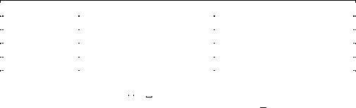
jointly zero with p-values are given in Table 6.1. The Wald statistics are asymptotically χ23 under the null hypothesis. Two versions of the asymptotic covariance matrix are estimated. Newey and West with 6 lags (denoted Wald(NW[6])), and Hansen-Hodrick with 2 lags (denoted Wald(HH[2])). In these data, UIP is rejected at reasonable levels of signiÞcance for every currency except for the dollar-deutschemark rate.

Table 6.1: Hansen-Hodrick tests of UIP

		US-BP US-JY US-DM			DM-BP DM-JY BP-JY
	Wald(NW[6])	16.23	400.47	5.701	66.77	46.35	294.31
	p-value	0.001	0.000	0.127	0.000	0.000	0.000
	Wald(HH[2])	16.44	324.85	4.299	57.81	32.73	300.24
	p-value	0.001	0.000	0.231	0.000	0.000	0.000

Notes: Regression st −ft−3,3 = z0t−3β +²t,3 estimated on monthly observations from 1973,3 to 1999,12. Wald is the Wald statistic for the test that β = 0. Asymptotic covariance matrix estimated by Newey-West with 6 lags (NW[6]) and by Hansen— Hodrick with 2 lags (HH[2]).

The Advantage of Using Overlapping Observations

The Hansen—Hodrick correction involves some extra work. Are the beneÞts obtained by using the extra observations worth the extra costs? Afterall, you can avoid inducing the serial correlation into the regression error by using nonoverlapping quarterly observations but then you would only have 111 data points. Using the overlapping monthly observations increases the nominal sample size by a factor of 3 but the e ective increase in sample size may be less than this if the additional observations are highly dependent.

166CHAPTER 6. FOREIGN EXCHANGE MARKET EFFICIENCY

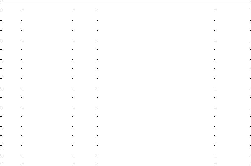
Table 6.2: Monte Carlo Distribution of OLS Slope Coe cients and T-ratios using Overlapping and Nonoverlapping Observations.

		Overlapping			percentiles		Relative
	T	Observations		2.5	50	97.5	Range
	50	yes	slope	0.778	0.999	1.207	0.471
			tNW	(-2.738)	(-0.010)	(2.716)	1.207
			tHH	[-2.998]	[-0.010]	[3.248]	1.383
	16	no	slope	0.543	0.998	1.453
			tOLS	((-2.228))	((-0.008))	((2.290))
	100	yes	slope	0.866	0.998	1.126	0.474
			tNW	(-2.286)	(-0.025)	(2.251)	1.098
			tHH	[-2.486]	[-0.020]	[2.403]	1.183
	33	no	slope	0.726	0.996	1.274
			tOLS	((-2.105))	((-0.024))	((2.026))
	300	yes	slope	0.929	1.001	1.074	0.509
			tNW	(-2.071)	(0.021)	(2.177)	1.041
			tHH	[-2.075]	[-0.016]	[2.065]	1.014
	100	no	slope	0.858	1.003	1.143
			tOLS	((-2.030))	((0.032))	((2.052))

Notes: True slope = 1. tNW : Newey—West t-ratio. tHH : Hansen—Hodrick t-ratio. tOLS: OLS t-ratio. Relative range is ratio of the distance between the 97.5 and 2.5 percentiles in the Monte Carlo distribution for the statistic constructed using overlapping observations to that constructed using nonoverlapping observations.

The advantage that one gains by going to monthly data are illus- (108) trated in table 6.2 which shows the results of a small Monte Carlo experiment that compares the two (overlapping versus nonoverlapping)

strategies. The data generating process is

yt+3 = xt + ²t+3,	iid
	²t N(0, 1),
xt = 0.8xt−1 + ut,	iid
	ut N(0, 1),

where T is the number of overlapping (monthly) observations. yt+3 is regressed on xt and Newey-West t-ratios tNW are reported in parentheses. 5 lags were used for T = 50, 100 and 6 lags used for T = 300.