1.1. INTERNATIONAL FINANCIAL MARKETS

9

British devaluation. Looking at an eleven-day window spanning the event an arbitrage that shorted 1 million pounds at a 1-month maturity could potentially have earned a 4521-pound proÞt on Wednesday November 24 at 7:30 a.m. but by 4:30 p.m. Thursday November 24, the proÞt opportunity had vanished. A second event that he looks at is the 1987 UK general election. Examining a window that spans from June 1 to June 19, proÞt opportunities were generally unavailable. Among the few opportunities to emerge was a quote at 7:30 a.m. Wednesday June 17 where a 1 million pound short position predicted 712 pounds of proÞt at a 1 month maturity. But by noon of the same day, the predicted proÞt fell to 133 pounds and by 4:00 p.m. the opportunities had vanished.

To summarize, the empirical evidence suggests that covered interest parity works pretty well. Occasional violations occur after accounting for transactions costs but they are short-lived and present themselves only during rare periods of high market volatility.

Uncovered Interest Parity

Let Et(Xt+1) = E(Xt+1|It) denote the mathematical expectation of the random variable Xt+1 conditioned on the date-t publicly available information set It. If foreign exchange participants are risk neutral, they care only about the mean value of asset returns and do not care at all about the variance of returns. Risk-neutral individuals are also willing to take unboundedly large positions on bets that have a positive expected value. Since Ft − St+1 is the proÞt from taking a position in forward foreign exchange, under risk-neutrality expected forward speculation proÞts are driven to zero and the forward exchange rate must, in equilibrium, be market participant’s expected future spot exchange rate

Ft = Et(St+1).

(1.6)

Substituting (1.6) into (1.2) gives the uncovered interest parity condition

	Et[St+1]
1 + it = (1 + i )		.	(1.7)
t	St

If (1.7) is violated, a zero-net investment strategy of borrowing in one currency and simultaneously lending uncovered in the other currency

10 CHAPTER 1. SOME INSTITUTIONAL BACKGROUND

has a positive payo in expectation. We use the uncovered interest parity condition as a Þrst-approximation to characterize international asset market equilibrium, especially in conjunction with the monetary model (chapters 3, 10, and 11). However, as you will see in chapter 6, violations of uncovered interest parity are common and they present an important empirical puzzle for international economists.

	Risk Premia. What reason can be given if uncovered interest parity
	does not hold? One possible explanation is that market participants
	are risk averse and require compensation to bear the currency risk in-
	volved in an uncovered foreign currency investment. To see the relation
	between risk aversion and uncovered interest parity, consider the fol-
	lowing two-period partial equilibrium portfolio problem. Agents take
	interest rate and exchange rate dynamics as given and can invest a frac-
(2)	tion α of their current wealth Wt in a nominally safe domestic bond
	with next period payo (1+it)αWt. The remaining 1−α of wealth can
	be invested uncovered in the foreign bond with future home-currency
	payo (1 + i )St+1 (1	−	α)W . We assume that covered interest parity
	t St		t
	is holds so that a covered investment in the foreign bond is equivalent
	to the investment in the domestic bond. Next period nominal wealth
	is the payo from the bond portfolio				¸ Wt.
	Wt+1 =	·α(1 + it) + (1 − α)(1 + it ) St t				(1.8)
				S +1

Domestic market participants have constant absolute risk aversion utility deÞned over wealth, U(W) = −e−γW where γ ≥ 0 is the coe cient of absolute risk aversion. The domestic agent’s problem is to choose the investment share α to maximize expected utility

Et[U(Wt+1)] = −Et ³e−γWt+1

´ .

(1.9)

Notice that the right side of (1.9) is the moment generating function of next period wealth.3

3The moment generating function for the normally distributed random variable

		¡	¢			σ2z2
	2	) is ψX (z) = E e	zX = e µz+			2	. Substituting W for X, −γ for z,
X N(µ, σ				2
W	for µ, and Var(Wt+1) for σ				and taking logs results in (1.12).
Et t+1					¡		¢

1.1. INTERNATIONAL FINANCIAL MARKETS

11

If people believe that Wt+1 is normally distributed conditional on currently available information, with conditional mean and conditional variance

				E St+1
EtWt+1 = ·α(1 + it) + (1 − α)(1 + it )				t			¸ Wt,			(1.10)
				St
(1		−	α)2(1 + i )2Var		(S	t+1		)W 2
Vart(Wt+1) =			t	t				t	.	(1.11)
			S2
			t

It follows that maximizing (1.9) is equivalent to maximizing the simpler

expression	γ
EtWt+1 −
	2 Var(Wt+1).	(1.12)

We say that traders are mean-variance optimizers. These individuals like high mean values of wealth, and dislike variance in wealth.

Di erentiating (1.12) with respect to α and re-arranging the Þrst-

order conditions for optimality yields

E [S

]

−

γW (1

−

α)(1 + i )2Var

(S

t+1

)

(1 + i

)

−

(1 + i )

t t+1

=

t

t

t

, (1.13)

St2

t

t

St

which implicitly determines the optimal investment share α. Even if there is an expected uncovered proÞt available, risk aversion limits the size of the position that investors will take. If all market participants are risk neutral, then γ = 0 and it follows that uncovered interest parity will hold. If γ > 0, violations of uncovered interest parity can occur and the forward rate becomes a biased predictor of the future spot rate, the reason being that individuals need to be paid a premium to bear foreign currency risk. Uncovered interest parity will hold if α = 1, regardless of whether γ > 0. However, the determination of α requires us to be speciÞc about the dynamics that govern St and that is information that we have not speciÞed here. The point that we want to make here is that the forward foreign exchange market can be in equilibrium and there are no unexploited risk-adjusted arbitrage proÞts even though the forward exchange rate is a biased predictor of the future spot rate. We will study deviations from uncovered interest parity in more detail in chapter 6.

12 CHAPTER 1. SOME INSTITUTIONAL BACKGROUND

Futures Contracts

Participation in the forward foreign exchange market is largely limited to institutions and large corporate customers owing to the size of the contracts involved. The futures market is available to individuals and is a close substitute to the forward market. The futures market is an institutionalized form of forward contracting. Four main features distinguish futures contracts from forward contracts.

First, foreign exchange futures contracts are traded on organized exchanges. In the US, futures contracts are traded on the International Money Market (IMM) at the Chicago Mercantile Exchange. In Britain, futures are traded at the London International Financial Futures Exchange (LIFFE). Some of the currencies traded are, the Australian dollar, Brazilian real, Canadian dollar, euro, Mexican peso, New Zealand dollar, pound, South African rand, Swiss franc, Russian ruble and the yen.

Second, contracts mature at standardized dates throughout the year. The maturity date is called the last trading day. Delivery occurs on the third Wednesday of March, June, Sept, and December, provided that it is a business day. Otherwise delivery takes place on the next business day. The last trading day is 2 business days prior to the delivery date. Contracts are written for Þxed face values. For example, for the face value of an euro contract is 125,000 euros.

Third, the exchange serves to match buyers to sellers and maintains a zero net position.4 Settlement between sellers (who take short positions) and buyers (who take long positions) takes place daily. You purchase a futures contract by putting up an initial margin with your broker. If your contract decreases in value, the loss is debited from your margin account. This debit is then used to credit the account of the individual who sold you the futures contract. If your contract increases in value, the increment is credited to your margin account. This settlement takes place at the end of each trading day and is called “marking to market.” Economically, the main di erence between futures and forward contracts is the interest opportunity cost associated with the

4If you need foreign exchange before the maturity date, you are said to have short exposure in foreign exchange which can be hedged by taking a long position in the futures market.

1.1. INTERNATIONAL FINANCIAL MARKETS

13

funds in the margin account. In the US, some part of the initial margin can be put up in the form of Treasury bills, which mitigates the loss of interest income.

Fourth, the futures exchange operates a clearinghouse whose function is to guarantee marking to market and delivery of the currencies upon maturity. Technically, the clearing house takes the other side of any transaction so your legal obligations are to the exchange. But as mentioned above, the clearinghouse maintains a zero net position.

Most futures contracts are reversed prior to maturity and are not held to the last trading day. In these situations, futures contracts are simply bets between two parties regarding the direction of future exchange rate movements. If you are long a foreign currency futures contract and I am short, you are betting that the price of the foreign currency will rise while I expect the price to decline. Bets in the futures market are a zero sum game because your winnings are my losses.

How a Futures Contract Works

For a futures contract with k days to maturity, denote the date T − k futures price by FT −k, and the face value of the contract by VT . The contract value at T − k is FT −kVT .

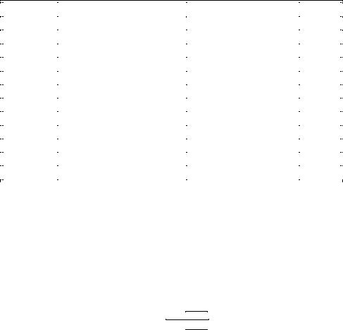
Table 1.1 displays the closing spot rate and the price of an actual 12,500,000 yen contract that matured in June 1999 (multiplied by 100) and the evolution of the margin account. When the futures price increases, the long position gains value as reßected by an increment in the margin account. This increment comes at the expense of the short position.

Suppose you buy the yen futures contract on June 16, 1998 at 0.007346 dollars per yen. Initial margin is 2,835 dollars and the spot exchange rate is 0.006942 dollars per yen. The contract value is 91,825 dollars. If you held the contract to maturity, you would take delivery of the 12,500,000 yen on 6/23/99 at a unit price of 0.007346 dollars. Suppose that you actually want the yen on December 17, 1998. You close out your futures contract and buy the yen in the spot market. The appreciation of the yen means that buying 12,500,000 yen costs 20675 dollars more on 12/17/98 than it did on 6/16/98, but most of the higher cost is o set by the gain of 21197.5-2835=18,362.5 dollars

14 CHAPTER 1. SOME INSTITUTIONAL BACKGROUND

Table 1.1: Yen futures for June 1999 delivery

					Long yen position
	Date	FT −k	ST −k	∆FT −k	∆(FT −kVT ) Margin		φT −k
	6/16/98	0.7346	0.6942	0.0000	0.0	2835.0	1.0581
	6/17/98	0.772	0.7263	0.0374	4675.0	7510.0	1.0628
	7/17/98	0.7507	0.7163	-0.0213	-2662.5	4847.5	1.0479
	8/17/98	0.7147	0.6859	-0.0360	-4500.0	347.5	1.0418
	9/17/98	0.7860	0.7582	0.0713	8912.5	9260.0	1.0365
	10/16/98	0.8948	0.8661	0.1088	13600.0	22860.0	1.0330
	11/17/98	0.8498	0.8244	-0.0450	-5625.0	17235.0	1.0308
	12/17/98	0.8815	0.8596	0.0317	3962.5	21197.5	1.0254
	01/19/99	0.8976	0.8790	0.0161	2012.5	23210.0	1.0211
	02/17/99	0.8524	0.8401	-0.0452	-5650.0	17560.0	1.0146
	03/17/99	0.8575	0.8463	0.0051	637.5	18197.5	1.0131

on the futures contract.

The hedge comes about because there is a covered interest paritylike relation that links the futures price to the spot exchange rate with eurocurrency rates as a reference point. Let iT −k be the Eurodollar rate at T −k which matures at T , iT −k be the analogous one-year Euroeuro rate, assume a 360 day year, and let

1 + kiT −k

φT−k = 360 , ki

1 + T −k

360

be the ratio of the domestic to foreign gross returns on an eurocurrency deposit that matures in k days. The parity relation for futures prices is

FT −k = φT −kST −k.

(1.14)

Here, the futures price varies in proportion to the spot price with φT−k being the factor of proportionality. As contract approaches last trading day, k → 0. It follows that φT −k → 1, and FT = ST . This means that you can obtain the foreign exchange in two equivalent ways. You can buy a futures contract on the last trading day and take delivery, or you