Chapter 3

The Monetary Model

The monetary model is central to international macroeconomic analysis and is a recurrent theme in this book. The model identiÞes a set of underlying economic fundamentals that determine the nominal exchange rate in the long run. The monetary model was originally developed as a framework to analyze balance of payments adjustments under Þxed exchange rates. After the breakdown of the Bretton Woods system the model was modiÞed into a theory of nominal exchange rate determination.

The monetary approach assumes that all prices are perfectly ßexible and centers on conditions for stock equilibrium in the money market. Although it is an ad hoc model, we will see in chapters 4 and 9 that many predictions of the monetary model are implied by optimizing models both in ßexible price and in sticky price environments. The monetary model also forms the basis for work on target zones (chapter 10) and in the analysis of balance of payments crises (chapter 11).

A note on notation: Throughout this chapter the level of a variable will be denoted in upper case letters and the natural logarithm in lower case. The only exception to this rule is that the level of the interest rate is always denoted in lower case. Thus it is the nominal interest rate and in logs, st is the nominal exchange rate in American terms, pt is the price level, yt is real income. Stars are used to denote foreign country variables.

79

80	CHAPTER 3. THE MONETARY MODEL

3.1Purchasing-Power Parity

A key building block of the monetary model is purchasing-power parity (PPP), which can be motivated according to the Casellian approach or by the commodity-arbitrage view.

Cassel’s Approach

The intellectual origins of PPP began in the early 1800s with the writings of Wheatly and Ricardo. These ideas were subsequently revived by Cassel [22]. The Casselian approach begins with the observation that the exchange rate S is the relative price of two currencies. Since the purchasing power of the home currency is 1/P and the purchasing power of the foreign currency is 1/P , in equilibrium, the relative value of the two currencies should reßect their relative purchasing powers,

S = P/P .

What is the appropriate deÞnition of the price level? The Casselian view suggests using the general price level. Whether the general price level samples prices of non-traded goods or not is irrelevant. As a result, the consumer price index (CPI) is typically used in empirical implementations of this theory. The following passage from Cassel is used by Frenkel [60] to motivate the use of the CPI in PPP research.

“Some people believe that Purchasing Power Parities should be calculated exclusively on price indices for such commodities as for the subject of trade between the two countries. This is a misinterpretation of the theory . . . The whole theory of purchasing power parity essentially refers to the internal value of the currencies concerned, and variations in this value can be measured only by general index Þgures representing as far as possible the whole mass of commodities marketed in the country.”

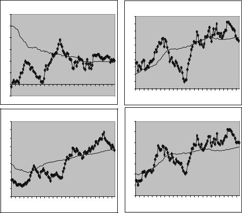
The theory implies that the log real exchange rate q ≡ s + p − p is constant over time. However, even casual observation rejects this prediction. Figure 3.1 displays foreign currency values of the US dollar and PPPs relative to four industrialized countries formed from CPIs

3.1. PURCHASING-POWER PARITY

81

1.2					US-UK
1
0.8
0.6
0.4
0.2
0
73	75	77	79	81	83	85	87	89	91	93	95	97
-0.2

1.4					US-Japan
1.2
1
0.8
0.6
0.4
0.2
0
-0.2
-0.4
73	75	77	79	81	83	85	87	89	91	93	95	97

					US-Germany
0.8
0.7
0.6
0.5
0.4
0.3
0.2
0.1
0
-0.1
-0.2
73	75	77	79	81	83	85	87	89	91	93	95	97

1.2				US-Switzerland
1
0.8
0.6
0.4
0.2
0
-0.2
73	75	77	79	81	83	85	87	89	91	93	95	97

Figure 3.1: Log nominal exchange rates (boxes) and CPI-based PPPs (solid).

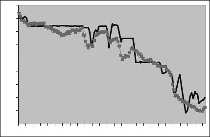
expressed in logarithms over the ßoating period. Figure 3.2 shows the analogous series for the US and UK over a long historical period extending from 1871 to 1997. While there are protracted periods in which the nominal exchange rate deviates from the PPP, the two series tend to revert towards each other over time.

As a result, international macroeconomists view Casselian PPP as a theory of the long-run determination of the exchange rate in which the PPP (p −p ) is a long-run attractor for the nominal exchange rate.

82	CHAPTER 3. THE MONETARY MODEL

60
40
20
0
-20
-40
-60	Nominal Exchange Rate (solid)
-80	PPPs from CPIs (boxes)
-100
-120
1871	1882	1893	1904	1915	1926	1937	1948	1959	1970	1981	1992

Figure 3.2: US—UK log nominal exchange rates and CPI-based PPPs multiplied by 100. 1871-1997.

The Commodity-Arbitrage Approach

The commodity-arbitrage view of PPP, articulated by Samuelson [124], simply holds that the law-of-one price holds for all internationally traded goods. Thus if the law-of-one price holds for the goods individually, it will hold for the appropriate price index as well. Here, the appropriate price index should cover only those goods that are traded internationally. It can be argued that the producer price index (PPI) is a better choice for studying PPP since it is more heavily weighted towards traded goods than the CPI which includes items such as housing services which do not trade internationally. We will consider empirical analyses on PPP in chapter 7.

PPP is clearly violated in the short run. Casual observation of Figures 3.1 and 3.2 suggest however that PPP may hold in the long run. There exists econometric evidence to support long-run PPP, but we will defer discussion of these issues until chapter 7.

In spite of the obvious short-run violations, PPP is one of the building blocks in the monetary model and as we will see in the Lucas model

3.2. THE MONETARY MODEL OF THE BALANCE OF PAYMENTS83

(chapter 4) and in the Redux model (chapter 9) as well. Why is that? (60) One reason frequently given is that we don’t have a good theory for why

PPP doesn’t hold so there is no obvious alternative way to provide international price level linkages. A second and perhaps more convincing reason is that all theories involve abstractions that are false at some level and as Friedman [64] argues, we should judge a theory not by the realism of its assumptions but by the quality of its predictions.

3.2The Monetary Model of the Balance of Payments

The Frenkel and Johnson [62] collection develops the monetary approach to the balance of payments under Þxed exchange rates. To illustrate the main idea, consider a small open economy that maintains a perfectly credible Þxed exchange rate s¯.1 it is the domestic nominal interest rate, Bt is the monetary base, Rt is the stock of foreign exchange reserves held by the central bank, Dt is domestic credit extended by the central bank. In logarithms, mt is the money stock, yt is national income, and pt is the price level. The money supply is Mt = µBt = µ(Rt +Dt) where µ is the money multiplier. A logarithmic expansion of the money supply and its components about their mean values allows us to write

mt = θrt + (1 − θ)dt

(3.1)

where θ = E(Rt)/E(Bt), rt = ln(Rt), and dt = ln(Dt).2

A transactions motive gives rise to the demand for money in which log real money demand mdt −pt depends positively on yt and negatively

on the opportunity cost of holding money it
			mtd − pt = φyt − λit + ²t.					(3.2)
1A small open economy takes world prices and world interest rates as given.
2A	Þrst-order		expansion		about	mean	values	gives
Mt − E(Mt) =		µ[Rt	− E(Rt)] + µ[Dt − E(Dt)]. But µ =				E(Mt)/E(Bt) where
Bt =	Rt + Dt	is the monetary base.			Now divide both sides by E(Mt) to get

[Mt − E(Mt)]/E(Mt) = θ[Rt − E(Rt)]/E(Rt) +(1 − θ)[Dt − E(Dt)]/E(Dt). Noting that for a random variable Xt, [Xt − E(Xt)]/E(Xt) ' ln(Xt) − ln(E(Xt)), apart from an arbitrary constant, we get (3.1) in the text.

84	CHAPTER 3. THE MONETARY MODEL

0 < φ < 1 is the income elasticity of money demand, 0 < λ is the

iid 2

interest semi-elasticity of money demand, and ²t (0, σ² ).

Assume that purchasing-power parity (PPP) and uncovered interest parity (UIP) hold. Since the exchange rate is Þxed, PPP implies that the price level pt = s¯+ pt is determined by the exogenous foreign price level. Because the Þx is perfectly credible, market participants expect no change in the exchange rate and UIP implies that the interest rate it = it is given by the exogenous foreign interest rate. Assume that the money market is continuously in equilibrium by equating mdt in (3.2) to mt in (3.1) and rearranging to get

θrt = s¯ + pt + φyt − λit − (1 − θ)dt + ²t.

(3.3)

(3.3) embodies the central insights of the monetary approach to the balance of payments. If the home country experiences any one or a combination of the following: a high rate of income growth, declining interest rates, or rising prices, the demand for nominal money balances will grow. If money demand growth is not satisÞed by an accommodating increase in domestic credit dt, the public will obtain the additional money by running a balance of payments surplus and accumulating international reserves. If, on the other hand, the central bank engages in excessive domestic credit expansion that exceeds money demand growth, the public will eliminate the excess supply of money by running a balance of payments deÞcit.

We will meet this model again in chapters 10 and 11 in the study of target zones and balance of payments crises. In the remainder of this chapter, we develop the model as a theory of exchange rate determination in a ßexible exchange rate environment.

3.3The Monetary Model under Flexible Exchange Rates

The monetary model of exchange rate determination consists of a pair of stable money demand functions, continuous stock equilibrium in the money market, uncovered interest parity, and purchasing-power parity.

3.3. THE MONETARY MODEL UNDER FLEXIBLE EXCHANGE RATES85

Under ßexible exchange rates, the money stock is exogenous. Equilibrium in the domestic and foreign money markets are given by

mt − pt	=	φyt − λit,	(3.4)
mt − pt	=	φyt − λit ,	(3.5)

where 0 < φ < 1 is the income elasticity of money demand, and λ > 0 is the interest rate semi-elasticity of money demand. Money demand parameters are identical across countries.

International capital market equilibrium is given by uncovered interest parity

it − it = Etst+1 − st,

(3.6)

where Etst+1 ≡ E(st+1|It) is the expectation of the exchange rate at

date t+1 conditioned on all public information It, available to economic (61) agents at date t.

Price levels and the exchange rate are related through purchasing-

power parity
st = pt − pt .	(3.7)

To simplify the notation, call

ft ≡ (mt − mt ) − φ(yt − yt )

the economic fundamentals. Now substitute (3.4), (3.5), and (3.6) into (3.7) to get

st = ft + λ(Etst+1 − st),	(3.8)
and solving for st gives
st = γft + ψEtst+1,	(3.9)
where

γ	≡	1/(1 + λ),
ψ	≡ λγ = λ/(1 + λ).

(3.9) is the basic Þrst-order stochastic di erence equation of the monetary model and serves the same function as an ‘Euler equation’ in optimizing models. It says that expectations of future values of the

86 CHAPTER 3. THE MONETARY MODEL

exchange rate are embodied in the current exchange rate. High relative money growth at home leads to a weakening of the home currency while high relative income growth leads to a strengthening of the home currency.

Next, advance time by one period in (3.9) to get st+1 = γft+1 +ψEt+1st+2. Take expectations conditional on time t infor-

mation and use the	law of iterated expectations	to get
Etst+1 = γEtft+1 + ψEtst+2 and substitute back into (3.9).		Now do
this again for st+2, st+3, . . . , st+k, and you get
k
jX	(ψ)jEtft+j + (ψ)k+1Etst+k+1.
st = γ		(3.10)
=0

Eventually, you’ll want to drive k → ∞ but in doing so you need to specify the behavior the term (ψ)kEtst+k.

The fundamentals (no bubbles) solution. Since ψ < 1, you obtain the unique fundamentals (no bubbles) solution by restricting the rate at which the exchange rate grows by imposing the transversality condition

lim (ψ)kEtst+k = 0,	(3.11)
k→∞

which limits the rate at which the exchange rate can grow asymptotically. If the transversality condition holds, let k → ∞ in (3.10) to get the present-value formula

∞
jX
st = γ (ψ)jEtft+j	(3.12)
=0

The exchange rate is the discounted present value of expected future values of the fundamentals. In Þnance, the present value model is a popular theory of asset pricing. There, s is the stock price and f is the Þrm’s dividends. Since the exchange rate is given by the same basic formula as stock prices, the monetary approach is sometimes referred to as the ‘asset’ approach to the exchange rate. According to this approach, we should expect the exchange rate to behave just like the prices of other assets such as stocks and bonds. From this perspective it will come as no surprise that the exchange rate more volatile than

3.3. THE MONETARY MODEL UNDER FLEXIBLE EXCHANGE RATES87

the fundamentals, just as stock prices are much more volatile than dividends. Before exploring further the relation between the exchange rate and the fundamentals, consider what happens if the transversality condition is violated.

Rational bubbles. If the transversality condition does not hold, it is possible for the exchange rate to be governed in part by an explosive bubble {bt} that will eventually dominate its behavior. To see why, let the bubble evolve according to

bt = (1/ψ)bt−1 + ηt,

(3.13)

iid 2

where ηt N(0, ση). The coe cient (1/ψ) exceeds 1 so the bubble process is explosive. Now add the bubble to the fundamental solution (3.12) and call the result

sˆt = st + bt.

(3.14)

You can see that sˆt violates the transversality condition by substituting (3.14) into (3.11) to get

ψt+kEtsˆt+k = ψt+kEtst+k +ψt+kEtbt+k = bt.

| {z }

0

However, sˆt is a solution to the model, because it solves (3.9). You can check this out by substituting (3.14) into (3.9) to get

st + bt = (ψ/λ)ft + ψ[EtSt+1 + (1/ψ)bt].

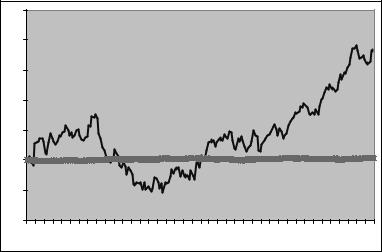
The bt terms on either side of the equality cancel out so sˆt is indeed is another solution to (3.9) but the bubble will eventually dominate and will drive the exchange rate arbitrarily far away from the fundamentals ft. The bubble arises in a model where people have rational expectations so it is referred to as a rational bubble. What does a rational bubble look like? Figure 3.3 displays a realization of a sˆt for 200 time periods where ψ = 0.99 and the fundamentals follow a driftless random walk with innovation variance 0.0352. Early on, the exchange rate seems to return to the fundamentals but the exchange rate diverges as time goes on.

88	CHAPTER 3. THE MONETARY MODEL

25
20
15
10					exchange rate
					with bubble
5
0
-5						fundamentals
-10
1	26	51	76	101	126	151	176

Figure 3.3: A realization of a rational bubble where ψ = 0.99, and the fundamentals follow a random walk. The stable line is the realization of the fundamentals.

Now it may be the case that the foreign exchange market is occasionally driven by bubbles but real-world experience suggests that such bubbles eventually pop. It is unlikely that foreign exchange markets are characterized by rational bubbles which do not pop. As a result, we will focus on the no-bubbles solution from this point on.

3.4Fundamentals and Exchange Rate Volatility

A major challenge to international economic theory is to understand the volatility of the exchange rate in relation to the volatility of the economic fundamentals. Let’s Þrst take a look at the stylized facts concerning volatility. Then we’ll examine how the monetary model is able to explain these facts.

3.4. FUNDAMENTALS AND EXCHANGE RATE VOLATILITY 89

Table 3.1: Descriptive statistics for exchange-rate and equity returns, and their fundamentals.

							Autocorrelations
		Mean	Std.Dev.	Min.	Max.	ρ1	ρ4	ρ8	ρ16
				Returns
	S&P	2.75	5.92	-13.34	18.31	0.24	-0.10	0.15	0.09
	UKP	0.41	5.50	-13.83	16.47	0.12	0.03	0.01	-0.29
	DEM	0.46	6.35	-13.91	15.74	0.09	0.23	0.04	-0.07
	YEN	0.73	6.08	-15.00 16.97		0.13 0.18 0.06 -0.29
			Deviation from fundamentals
	Div.	1.31	0.30	0.49	1.82	1.01	1.03	1.05	0.94
	UKP	0	0.18	-0.46	0.47	0.89	0.61	0.25	-0.12
	DEM	0	0.31	-0.61	0.59	0.98	0.91	0.77	0.55
	YEN	0	0.38	-0.85	0.50	0.98	0.88	0.76	0.68

Notes: Quarterly observations from 1973.1 to 1997.4. Percentage returns on the Standard and Poors composite index (S&P) and its log dividend yield (Div.) are from Datastream. Percentage exchange rate returns and deviation of exchange rate from fundamentals (st−ft) with ft = (mt−mt )−(yt−yt ) are from the International Financial Statistics CD-ROM. (st −ft) are normalized to have zero mean. The US dollar is the numeraire currency. UKP is the UK pound, DEM is the deutschemark, and YEN is the Japanese yen.

Stylized Facts on Volatility and Dynamics.

Some descriptive statistics for dollar quarterly returns on the pound, deutsche-mark, yen are shown in the Þrst panel of Table 3.1. To underscore the similarity between the exchange rate and equity prices, the table also includes statistics for the Standard and Poors composite stock price index. The second panel displays descriptive statistics for the deviation of the respective asset prices from their fundamentals. For equities, this is the S&P log dividend yield. For currency values, it

is the deviation of the exchange rate from the monetary fundamentals, (62) ft − st have been normalized to have mean 0. The volatility of a time

series is measured by its sample standard deviation.

90	CHAPTER 3. THE MONETARY MODEL

The main points that can be drawn from the table are

1.The volatility of exchange rate returns ∆st is virtually indistinguishable from stock return volatility.

2.Returns for both stocks and exchange rates have low Þrst-order serial correlation.

3.From our discussion about the properties of the variance ratio statistic in chapter 2.4, the negative autocorrelations in exchange rate returns at 16 quarters suggest the possibility of mean reversion.

4.The deviation of the price from the fundamentals display substantial persistence, and much less volatility than returns. The behavior of the dividend yield, while similar to the behavior of the exchange rate deviations from the monetary fundamentals, displays slightly more persistence and appears to be nonstationary over the sample period.

The data on returns and deviations from the fundamentals are shown in Figure 3.4 where you clearly see how the exchange rate is excessively volatile in comparison to its fundamentals.

Excess Volatility and the Monetary Model

The monetary model can be made consistent with the excess volatility in the exchange rate if the growth rate of the fundamentals is a persistent stationary process.

iid

∆ft = ρ∆ft−1 + ²t.

(3.15)

2

The implied k−step ahead prediction formulae

(63)

with ²t

N(0, σ²k).

are E (∆f

) = ρ ∆f . Converting to levels, you get E (f

) = f +

P

k

t i

t+k

tk

t t+k

t

i=1

ρ ∆ft = ft+[(1−ρ )/(1−ρ)]ρ∆ft. Using these prediction formulae

in (3.12) gives

∞

∞

ψj

∞

(ρψ)j

jX

X

X

st

1

−

ρρ∆ft − γ

1

−

ρ ρ∆ft

= γ

ψjft + γ

j=0

=0

j=0

ρψ

= ft +

∆ft,

(3.16)

1 − ρψ