158 CHAPTER 5. INTERNATIONAL REAL BUSINESS CYCLES

and investment rates are
˜	=	˜	− (1	−	˜	(5.58)
it		γkt+1			δ)kt,
˜	=	˜	− (1	−	˜	(5.59)
it		γkt+1			δ)kt .
Let world consumption be c˜tw		= c˜t + c˜t		= y˜t + y˜t − (˜it + ˜it ). By the
		t		−		t
optimal risk-sharing rule (5.39) c˜ = [(1					ω)/ω]˜c , which can be used
to determine
		c˜t = ωc˜tw.				(5.60)

It follows that c˜t = c˜wt − c˜t. The log-level of consumption is recovered by

ln(Ct) = ln(Xt) + ln(˜ct + c).

Log levels of the other variables can be obtained in an analogous manner.

Simulating the Two-Country Model

The steady state values are

y = y = 1.53, k = k = 3.66, i = i = 0.42, c = c = 1.11.

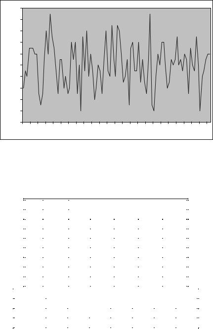
The model is used to generate 96 time-series observations. Descriptive statistics calculated using the Hodrick—Prescott Þltered cyclical parts of the log-levels of the simulated observations and are displayed in Table 5.4 and Figure 5.4 shows the simulated current account balance.

The simple model of this chapter makes many realistic predictions.

It produces time-series that are persistent and that display coarse comovements that are broadly consistent with the data. But there are also several features of the model that are inconsistent with the data. First, consumption in the two-country model is smoother than output. Second, domestic and foreign consumption are perfectly correlated due to the perfect risk-sharing whereas the correlation in the data is much lower than 1. A related point is that home and foreign output are predicted to display a lower degree of co-movement than home and foreign consumption which also is not borne out in the data.

5.2. CALIBRATING A TWO-COUNTRY MODEL

159

0.1
0.08
0.06
0.04
0.02
0
-0.02
-0.04
-0.06
-0.08
-0.1
73	75	77	79	81	83	85	87	89	91	93	95	97

Figure 5.4: Simulated current account to GDP ratio.

Table 5.4: Calibrated Open-Economy Model

				Std.		Autocorrelations
				Dev.	1	2		3		4				6
		yt	0.022		0.66	0.40		0.15		0.07			0.04
		ct	0.017		0.63	0.42		0.18		0.12			-0.04
		it	0.114		0.05	-0.13		-0.09		-0.10			0.03
		ext	0.038		0.09	-0.09		-0.09		-0.10			-0.00
		yt	0.021		0.65	0.32		0.07		-0.15			-0.27
		ct	0.017		0.63	0.42		0.18		0.12			-0.04
		it	0.116		0.03	-0.15		-0.07		-0.08			0.00
					Cross correlations at k
				6	4	1		0	-1				-4		-6
extyt−k				0.00	0.18	0.41		0.44	0.21			0.15			0.15
yt yt−k				0.10	0.06	0.27		0.18	0.06			0.28			0.05

160 CHAPTER 5. INTERNATIONAL REAL BUSINESS CYCLES

International Real Business Cycles Summary

1.The workhorse of real business cycle research is the dynamic stochastic general equilibrium model. These can be viewed as Arrow-Debreu models and solved by exploiting the social planner’s problem. They feature perfect markets and completely fully ßexible prices. The models are fully articulated and are have solidly grounded micro foundations.

2.Real business cycle researchers employ the calibration method to quantitatively evaluate their models. Typically, the researcher takes a set of moments such as correlations between actual time series, and asks if the theory is capable of replicating these comovements. The calibration style of research stands in contrast with econometric methodology as articulated in the Cowles commission tradition. In standard econometric practice one begins by achieving model identiÞcation, progressing to estimation of the structural parameters, and Þnally by conducting hypothesis tests of the model’s overidentifying restrictions but how one determines whether the model is successful or not in the calibration tradition is not entirely clear.