11.2. A SECOND GENERATION MODEL

335

11.2A Second Generation Model

In Þrst-generation models, exogenous domestic credit expansion causes international reserves to decline in order to maintain a constant money supply that is consistent with the Þxed exchange rate. A key feature of second generation models is that they explicitly account for the policy options available to the authorities. To defend the exchange rate, the government may have to borrow foreign exchange reserves, raise domestic interest rates, reduce the budget deÞcit and/or impose exchange controls. Exchange rate defense is therefore costly. The government’s willingness to bear these costs depend in part on the state of the economy. Whether the economy is in the good state or in the bad state in turn depends on the public’s expectations. The government engages in a cost-beneÞt calculation to decide whether to defend the exchange rate or to realign.

We will study the canonical second generation model due to Obstfeld [112]. In this model, the government’s decision rule is nonlinear and leads to multiple (two) equilibria. One equilibrium has low probability of devaluation whereas the other has a high probability. The costs to the authorities of maintaining the Þxed exchange rate depend on the public’s expectations of future policy. An exogenous event that changes the public’s expectations can therefore raise the government’s assessment of the cost of exchange rate maintenance leading to a switch from the low-probability of devaluation equilibrium to the high-probability of devaluation equilibrium.

What sorts of market-sentiment shifting events are we talking about? Obstfeld o ers several examples that may have altered public expectations prior to the 1992 EMS crisis: The rejection by the Danish public of the Maastrict Treaty in June 1992, a sharp rise in Swedish unemployment, and various public announcements by authorities that suggested a weakening resolve to defend the exchange rate. In regard to the Asian crisis, expectations may have shifted as information about over-expansion in Thai real-estate investment and poor investment allocation of Korean Chaebol came to light.

336 CHAPTER 11. BALANCE OF PAYMENTS CRISES

Obstfeld’s Multiple Devaluation Threshold Model

All variables are in logarithms. Let pt be the domestic price level and st be the nominal exchange rate. Set the (log) of the exogenous foreign price level to zero and assume PPP, pt = st. Output is given by a quasi-labor demand schedule which varies inversely with the real wage

iid
wt − st, and with a shock ut N(0, σu2)
yt = −α(wt − st) − ut.	(11.23)

Firms and workers agree to a rule whereby today’s wage was negotiated and set one-period in advance so as to keep the ex ante real wage constant

wt = Et−1(st).

(11.24)

Optimal Exchange Rate Management

We Þrst study the model where the government actively manages, but does not actually Þx the exchange rate. The authorities are assumed to have direct control over the current-period exchange rate.

The policy maker seeks to minimize costs arising from two sources. The Þrst cost is incurred when an output target is missed. Notice that (11.23) says that the natural output level is Et−1(yt) = 0. We assume that there exists an entrenched but unspeciÞed labor market distortion that prevents the natural level of output from reaching the socially e cient level. These distortions create an incentive for the government to try to raise output towards the e cient level. The government sets a target level of output y¯ > 0. When it misses the output target, it bears a cost of (¯y − yt)2/2 > 0.

The second cost is incurred when there is inßation. Under PPP with the foreign price level Þxed, the domestic inßation rate is the depreciation rate of the home currency, δt ≡ st −st−1. Together, policy errors generate current costs for the policy maker `t, according to the

quadratic loss function
`t =	θ		(δt)2 +	1	[¯y	− yt]2.	(11.25)
	2			2

Presumably, it is the public’ desire to minimize (11.25) which it achieves by electing o cials to fulÞll its wishes.

11.2. A SECOND GENERATION MODEL

337

The static problem is the only feasible problem. In an ideal world, the government would like to choose current and future values of the

exchange rate to minimize the expected present value of future costs (225)

Et X∞ βj`t+j, j=0

where β < 1 is a discount factor. The problem is that this opportunity is not available to the government because there is no way that the authorities can credibly commit themselves to pre-announced future actions. Future values of st are therefore not part of the government’s current choice set. The problem that is within the government’s ability to solve is to choose st each period to minimize (11.25), subject to (11.24) and (11.23). This boils down to a sequence of static problems so we omit the time subscript from this point on.

Let s0 be yesterday’s exchange rate and E0(s) be the public’s expectation of today’s exchange rate formed yesterday. The government Þrst observes today’s wage w = E0(s), and today’s shock u, then chooses today’s exchange rate s to minimize ` in (11.25). The optimal exchangerate management rule is obtained by substituting y from (11.23) into (11.25), di erentiating with respect to s and setting the result to zero. Upon rearrangement, you get the government’s reaction function

s = s0 +	α	[α(w − s) + y¯ + u] .	(11.26)
	θ

Notice that the government’s choice of s depends on yesterday’s prediction of s by the public since w = E0(s). Since the public knows that the government follows (11.26), they also know that their forecasts of the future exchange rate partly determine the future exchange rate. To solve for the equilibrium wage rate, w = E0(s), take expectations of (11.26) to get

w = s0 +	αy¯
	θ .	(11.27)

To cut down on the notation, let

α2 λ = θ + α2 .

338	CHAPTER 11.	BALANCE OF PAYMENTS CRISES
Now, you can get the rational expectations equilibrium depreciation
rate by substituting (11.27) into (11.26)							(226)
	δ =		αy¯	+	λu	.	(11.28)
			θ		α

The equilibrium depreciation rate exhibits a systematic bias as a result of the output distortion y¯.3. The government has an incentive to set y = y¯. Seeing that today’s nominal wage is predetermined, it attempts to exploit this temporary rigidity to move output closer to its target value. The problem is that the public knows that the government will do this and they take this behavior into account in setting the wage. The result is that the government’s behavior causes the public to set a wage that is higher than it would set otherwise.

Fixed Exchange Rates

The foregoing is an analysis of a managed ßoat. Now, we introduce a reason for the government to Þx the exchange rate. Assume that in addition to the costs associated with policy errors given in (11.25), the government pays a penalty for adjusting the exchange rate. Where does this cost come from? Perhaps there are distributional e ects associated with exchange rate changes where the losers seek retribution on the policy maker. The groups harmed in a revaluation may di er from those harmed in a devaluation so we want to allow for di erential costs associated with devaluation and revaluation.4 So let cd be the cost associated with a devaluation and cr be the cost associated with a revaluation. The modiÞed current-period loss function is

` =	θ		(δ)2 +	1	(¯y	− y)2 + cdzd + crzr,	(11.29)
	2			2

where zd = 1 if δ > 0 and is 0 otherwise, and zr = 1 if δ < 0 and is zero otherwise. We also assume that the central bank either has su cient

3This is the inßationary bias that arises in Barro and Gordon’s [7] model of monetary policy

4Devaluation is an increase in s which results in a lower foreign exchange value of the domestic currency. Revaluation is a decrease in s, which raises the foreign exchange value of the domestic currency.

11.2. A SECOND GENERATION MODEL

339

reserves to mount a successful defense or has access to su cient lines of credit for that purpose.

The government now faces a binary choice problem. After observing the output shock u and the wage w it can either maintain the Þx or realign. To decide the appropriate course of action, compute the costs associated with each choice and take the low-cost route.

Maintenance costs. Suppose the exchange rate is Þxed at s0. The expected rate of depreciation is δe = E0(s) − s0. If the government maintains the Þx, adjustment costs are cd = cr = 0, and the depreci-

ation	rate is δ = 0. Substituting real wage w					−	s	= δe	and output
		e						0
y = −αδ			− u into (11.29) gives the cost to the policy maker of main-
taining the Þx				1
			`M =		[αδe + y¯ + u]2 .				(11.30)
				2

Realignment Costs. If the government realigns, it does so according to the optimal realignment rule (11.26) with a devaluation given by

δ =	α	[α(w − s) + y¯ + u].	(11.31)
	θ

Add and subtract (α2/θ)s0 to the right side of (11.31). Noting that δe = w − s0 and collecting terms gives

	δ =		λ		[αδe + y¯ + u] .		(11.32)
			α
Equating (11.31) and (11.32) you get the real wage
w	−	s =			θδe − α(¯y + u)	.	(11.33)
					α2 + θ

Substitute (11.33) into (11.23) to get the deviation of output from the

	target	θ
	y¯ − y =		[αδe + y¯ + u] .	(11.34)
		θ + α2

Substitute (11.32) and (11.34) into (11.29) to get the cost of realignment

			θ			[αδe		+ y¯ + u]2 + cd	if	u > 0
			2
`R =		2(θ	+α )				e	2		.	(11.35)
			θ			[αδ			if
		2(θ+α2)						+ y¯ + u] + cr		u < 0

340	CHAPTER 11. BALANCE OF PAYMENTS CRISES

Realignment rule. A realignment will be triggered if `R < `M . The central bank devalues if u > 0 and 2cd > λ[αδe + y¯ + u]2. It will and revalue if u < 0 and 2cr > λ[αδe + y¯ + u]2. The rule can be written more compactly as

λ[αδe + y¯ + u]2 > 2ck,

(11.36)

where k = d if u > 0 and k = r if u < 0. The realignment rule is sometimes called an escape-clause arrangement. There are certain extreme conditions under which everyone agrees that the authorities should escape the Þxed exchange-rate arrangement. The realignment costs cd, cr are imposed to ensure that during normal times the authorities have the proper incentive to maintain the exchange rate and therefore price stability.

Central bank decision making given δe. Let’s characterize the realignment rule for a given value of the public’s devaluation expectations δe. By (11.36), large positive realizations of u are big negative hits to output and trigger a devaluation. Large negative values of u are big positive output shocks and trigger a revaluation.

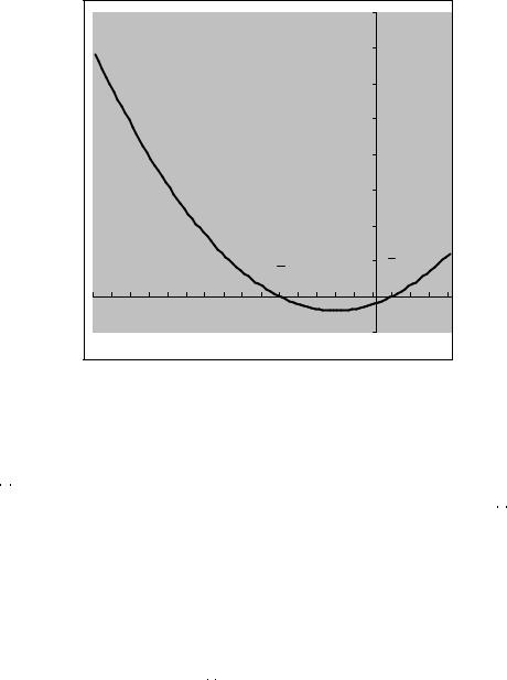
(11.36) is a piece-wise quadratic equation. For positive realizations of u, you want to Þnd the critical value u¯ such that u > u¯ triggers a devaluation. Write (11.36) as an equality, set ck = cd, and solve for the roots of the equation. You are looking for the positive devaluation trigger point so ignore the negative root because it is irrelevant. The

positive root is
u¯ = −αδe − y¯ + s	2λcd .	(11.37)

Now do the same for negative realizations of u, and throw away the positive root. The lower trigger point is

s

u = −αδe − y¯ − 2λcd . (11.38)

The points [u, u¯] are those that trigger the escape option. Realizations of u in the band [u, u¯] result in maintenance of the Þxed exchange rate. Figure 11.2 shows the attack points for δe = 0.03 with y¯ = 0.01, α = 1, θ = 0.15, cr = cd = 0.0004.

11.2. A SECOND GENERATION MODEL

341

							0.016
							0.014
							0.012
							0.01
							0.008
							0.006
							0.004
					u		0.002	u
							0
-0.15	-0.13	-0.11	-0.09	-0.07	-0.05	-0.03	-0.01	0.01	0.03
							-0.002

Figure 11.2: Realignment thresholds for given δe.

Multiple trigger points for devaluation.

u and u¯ depend on δe. But the public also forms its expectations conditional on the devaluation trigger points. This means that u, u¯ and δe must be solved simultaneously.

To simplify matters, we restrict attention to the case where the government may either defend the Þx or devalue the currency. Revaluation is not an option. We therefore focus on the devaluation threshold u¯. We will set cr to be a very large number to rule out the possibility of a revaluation. The central bank’s devaluation rule is

δ =	( δ1	=	αλ	[αδe + y¯ + u]	if	u > u¯ .	(11.39)
	δ0	=	0		if	u < u¯

Let P[X = x] be the probability of the event X = x. The expected depreciation is

δe = E0(δ)

342CHAPTER 11. BALANCE OF PAYMENTS CRISES

=P[δ = δ0]δ0 + P[δ = δ1]E[(λ/α)(αδe + y¯ + E(u|u > u¯))]

=P[u > u¯](λ/α)[αδe + y¯ + E(u|u > u¯)].

Solving for δe as a function of u¯ yields

δe =

λP(u > u¯) 1

[¯y + E(u|u > u¯)] .

(11.40)

1 − λP(u > u¯)

α

To proceed further, you need to assume a probability law governing the

output shocks, u.

Uniformly distributed output shocks. Let u be uniformly distributed on

the interval [−a, a].

The

probability density

function

of u is

f(u) = 1/(2a) for −a < u < a and the conditional density given u > u¯

is, g(u|u > u¯) = 1/(a − u¯). It follows that

P(u > u¯) = Zu¯a(1/(2a))dx =

(a

− u¯)

,

(11.41)

2a

a

(a + u¯)

E(u|u > u¯) = Zu¯

x/(a − u¯)dx =

.

(11.42)

2

Substituting (11.41) and (11.42) into (11.40) gives

a+¯u

.

δe = fδ(¯u) =

λ(a − u¯)

y¯ + 2

(11.43)

λ(a u¯)

2αa

1 −

2−a

Notice that δe involves the square terms u¯2. Quadratic equations usu-

ally have two solutions. Substituting δe into (11.37) gives

y¯ + s

u¯ =

−

αfδ

(¯u)

−

2cd

,

(11.44)

λ

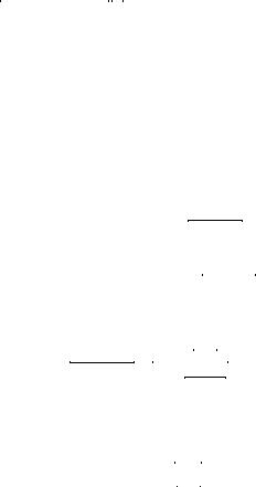
where fδ(¯u) is deÞned in (11.43). (11.44) has two solutions for u¯, each

of which trigger a devaluation. For parameter values a = 0.03, θ = 0.15,

c = 0.0004, α = 1, y¯ = 0.01 solving (11.44) yields the two solutions

(229)

u¯1 = −0.0209 and u¯2 = 0.0030. (11.44) is displayed in Figure 11.3 for

these parameter values.

Using (11.43), the public’s expected depreciation associated with u¯1

is 2.7 percent whereas δe

associated with u¯2 is 45 percent. The high

11.2. A SECOND GENERATION MODEL

343

			0.02
			0.015
			0.01
			0.005
			0
-0.03	-0.02	-0.01	0.00	0.01	0.02
			-0.005

Figure 11.3: Multiple equilibria devaluation thresholds.

expected inßation (high δe) gets set into wages and the resulting wage inßation increases the pain from unemployment and makes devaluation more likely. Devaluation is therefore more likely under the equilibrium threshold u¯2 than u¯1. When perceptions switch the economy to u¯2, the authorities require a very favorable output shock in order to maintain the exchange rate.

There is not enough information in the model for us to say which of the equilibrium thresholds the economy settles on. The model only suggests that random events can shift us from one equilibrium to another, moving from one where devaluation is viewed as unlikely to one in which it is more certain. Then, a relatively small output shock can suddenly trigger a speculative attack and subsequent devaluation.

344	CHAPTER 11. BALANCE OF PAYMENTS CRISES

Balance of Payments Crises Summary

1.A Þxed exchange rate regime will eventually collapse. The result is typically a balance of payments or currency crisis characterized by substantial Þnancial market volatility and large losses of foreign exchange reserves by the central bank.

2.Prior to the 1990s, crises were seen mainly to be the result of bad macroeconomic management–policies choices that were inconsistent with the long-run maintenance of the exchange rate. First-generation models focused on predicting when a crisis might occur. These models suggest that macroeconomic fundamentals such as the budget deÞcit, the current account deÞcit and external debt relative to the stock of international reserves should have predictive content for future crises.

3.Second-generation models are models of self-fulÞlling crises which endogenize government policy making and emphasize the interaction between the authorities’s decisions and the public’s expectations. Sudden shifts in market sentiment can weaken the government’s willingness to maintain the exchange rate which thereby triggers a crisis.