4.4. INTRODUCTION TO THE CALIBRATION METHOD 125

4.4Introduction to the Calibration Method

The Lucas model plays a central role in asset-pricing research. Chapter 6 covers some tests of its predictions using time-series econometric methods. At this point we introduce an alternative and popular methodology called calibration. In the calibration method, the researcher simulates the model given ‘reasonable’ values to the underlying taste and technology parameters and looks to see whether the simulated observations match various features of the real-world data.

Because there is no capital accumulation or production, the technology in the Lucas model is a stochastic process governing the evolution of xt and yt. The reasonably simple mechanics underlying the model makes its calibration relatively straightforward. Our work here will set the stage for the next chapter as real business cycle researchers rely heavily on the calibration method to evaluate the performance of their models.

Cooley and Prescott [33] set out the ingredients of the calibration method proceeds as follows.

1.Obtain a set of measurements from real-world data that we want to explain. These are typically a set of sample moments such

as the mean, the standard deviation, and autocorrelations of a time-series. Special emphasis is often placed on the crosscorrelations between two series which measure the extent of their co-movements.

2.Solve and calibrate a candidate model. That is, assign values to the deep parameters of tastes (the utility function) and technology (the production function) that make sense or that have been estimated by others.

3.Run (simulate) the model by computer and generate time-series of the variables that we want to explain.

4.Decide whether the computer generated time-series implied by the model ‘look like’ the observations that you want to explain.6

6The standard analysis is not based on classical statistical inference, although

126	CHAPTER 4. THE LUCAS MODEL

4.5Calibrating the Lucas Model

Measurement. The measurements that we ask the Lucas model to match are the volatility (standard deviation) and Þrst-order autocorrelation of the gross rate of depreciation, St+1/St, the forward premium Ft/St, the realized forward proÞt (Ft − St+1)/St, and the slope coe - cient from regressing the gross depreciation on the forward premium. Using quarterly data for the U.S. and Germany from 1973.1 to 1997.1, the measurements are given in the row labeled ‘data’ in Table 4.2.

Table 4.2: Measured and Implied Moments, US-Germany

			Volatility		Autocorrelation
	Slope	St+1	Ft	(Ft−St+1)	St+1	Ft	(Ft−St+1)
		St	St	St	St	St	St
Data	-0.293	0.060	0.008	0.061	0.007	0.888	0.026
Model	-1.444	0.014	0.006	0.029	0.105	0.006	0.628

Note: Model values generated with γ = 10, θ = 0.5.

The implied forward and spot exchange rates exhibit the so-called forward premium puzzle–that the forward premium predicts the future depreciation, but with a negative sign. Recall that the uncovered interest parity condition implies that the forward premium predicts the future depreciation with a coe cient of 1. The depreciation and the realized proÞt exhibit volatility of similar magnitude which is much larger than the volatility of the forward premium. All three series exhibit substantial serial dependence.

Calibration. Let random variables be denoted with a ‘tilde.’ The ‘technology’ that underlies the model are the exogenous monetary growth

˜ ˜

rates λ, λ , and the exogenous output growth rates g,˜ g˜ . Let the state

˜ ˜ ˜

vector be φ = (λ, λ , g,˜ g˜ ). The process governing the state vector is a Þnite-state Markov chain with stationary probabilities (see the chapter

Cecchetti et.al. [24], Burnside [18], Gregory and Smith [67] show how calibration methods can be combined with classical statistical inference, but the practice has not caught on.

4.5. CALIBRATING THE LUCAS MODEL

127

appendix). Each element of the state vector is allowed to be in either of one of two possible states—high and low. A ‘1’ subscript indicates that the variable is in the high growth state and a ‘2’ subscript indicates that the variable is in the low growth state. Therefore, λ = λ1 indicates high domestic money growth, λ = λ2 indicates low domestic money growth. Analogous designations hold for the other variables. The 16 possible states of the world are

φ	1 = (λ1, λ1, g1, g1)			φ			9 = (λ2, λ1, g1, g1)
φ	2 = (λ1, λ1, g1, g2)		φ			10 = (λ2, λ1, g1, g2)
φ	3 = (λ1, λ1, g2, g1)		φ			11 = (λ2, λ1, g2, g1)
φ4 = (λ1, λ1, g2, g2)			φ12 = (λ2, λ1, g2, g2)
φ	5 = (λ1, λ2, g1, g1)		φ			13 = (λ2, λ2, g1, g1)
φ	6 = (λ1, λ2, g1, g2)		φ			14 = (λ2, λ2, g1, g2)
φ	7 = (λ1, λ2, g2, g1)		φ			15 = (λ2, λ2, g2, g1)
φ	8 = (λ1, λ2, g2, g2)	φ			16 = (λ2, λ2, g2, g2).

We will denote the 16 × 16 probability transition matrix for the state

˜

φ

j|

˜

φ

i] the ij−th element.

by P, where pij = P[

φ

t+1 =

φ

t

=

The price

of the

domestic

and foreign currency bonds are,

bt

= βEt[(gθ

g (1−θ))1−γ]/λt+1,

and b

= βEt[(gθ

g (1−θ))1−γ]/λ

,

t+1

t+1

t

t+1

t+1

t+1

under the constant relative risk aversion utility function (4.22). Since their values depend on the state of the world, we say that these are state-contingent bond prices. Next, deÞne G = [(gθg (1−θ))1−γ]/λ and G = [(gθg (1−θ))1−γ]/λ , and let d = λ/λ be the gross rate of depreciation of the home currency. The possible values of G and G and d are given in Table 4.3,

Suppose the current state is φk. By (4.56), the spot exchange rate

is given

by (1

−

θ)d

k

/θ. The domestic bond price is

16

16

bk = β

i=1 pk,iGi, the foreign bond price is bk = β

i=1 pk,iGi , the

expected gross change in the nominal exchange rate is

16

p d

, and

P

P i=1

k,i i

the state-k contingent risk premium is

P

16

( 16

pk,iG )

Xi

i=1

i

rpk = =1 pk,idi −

(Pi16=1 pk,iGi)

.

P

Next, we must estimate the probability transition matrix. The Þrst question is whether we should use consumption data or GDP? In the

128						CHAPTER 4. THE LUCAS MODEL
				Table 4.3: Possible State Values
	G1	= [(gθg (1−θ))1−γ]/λ1			G	= [(gθg (1−θ))1−γ]/λ					d1	= λ1	/λ
			1	1	1		1		1	1				1
	G2	= [(gθg (1−θ))1−γ]/λ1			G	= [(gθg (1−θ))1−γ]/λ					d2	= λ1	/λ
			1	2	2		1		2	1				1
	G3	= [(gθg (1−θ))1−γ]/λ1			G	= [(gθg (1−θ))1−γ]/λ					d3	= λ1	/λ
			2	1	3		2		1	1				1
	G4	= [(gθg (1−θ))1−γ]/λ1			G	= [(gθg (1−θ))1−γ]/λ					d4	= λ1	/λ
			2	2	4		2		2	1				1
	G5	= [(gθg (1−θ))1−γ]/λ1			G	= [(gθg (1−θ))1−γ]/λ					d5	= λ1	/λ
			1	1	5		1		1	2				2
	G6	= [(gθg (1−θ))1−γ]/λ1			G	= [(gθg (1−θ))1−γ]/λ					d6	= λ1	/λ
			1	2	6		1		2	2				2
	G7	= [(gθg (1−θ))1−γ]/λ1			G	= [(gθg (1−θ))1−γ]/λ					d7	= λ1	/λ
			2	1	7		2		1	2				2
	G8	= [(gθg (1−θ))1−γ]/λ1			G	= [(gθg (1−θ))1−γ]/λ					d8	= λ1	/λ
			2	2	8		2		2	2				2
	G9	= [(gθg (1−θ))1−γ]/λ2			G	= [(gθg (1−θ))1−γ]/λ					d9	= λ2	/λ
			1	1	9		1		1	1				1
	G10		= [(gθg (1−θ))1−γ]/λ2		G		= [(gθg (1−θ))1−γ]/λ				d10 = λ2			/λ
			1	2	10			1	2	1				1
	G11		= [(gθg (1−θ))1−γ]/λ2		G		= [(gθg (1−θ))1−γ]/λ				d11 = λ2			/λ
			2	1	11			2	1	1				1
	G12		= [(gθg (1−θ))1−γ]/λ2		G		= [(gθg (1−θ))1−γ]/λ				d12 = λ2			/λ
			2	2	12			2	2	1				1
	G13		= [(gθg (1−θ))1−γ]/λ2		G		= [(gθg (1−θ))1−γ]/λ				d13 = λ2			/λ
			1	1	13			1	1	2				2
	G14		= [(gθg (1−θ))1−γ]/λ2		G		= [(gθg (1−θ))1−γ]/λ				d14 = λ2			/λ
			1	2	14			1	2	2				2
	G15		= [(gθg (1−θ))1−γ]/λ2		G		= [(gθg (1−θ))1−γ]/λ				d15 = λ2			/λ
			2	1	15			2	1	2				2
	G16		= [(gθg (1−θ))1−γ]/λ2		G		= [(gθg (1−θ))1−γ]/λ				d16 = λ2			/λ
			2	2	16			2	2	2				2

Lucas model, consumption equals GDP so there is no theoretical presumption as to which series we should use. Since prices depend on utility which depends on consumption. From this perspective, it makes sense to use consumption data which is what we do. The consumption and money data are from the International Financial Statistics and are in per capita terms.

The next question is what estimation technique to use? Using generalized method of moments or simulated method of moments (see chapter 2.2.2 and chapter 2.2.3) to estimate the transition matrix might be good choices if the dimensionality of the problem were smaller. Since we don’t have a very long time span of data, it turns out that estimating the transition probability matrix P by GMM or by the SMM does not work well. Instead, we ‘estimate’ the transition probabilities by counting the relative frequency of the transition events.

Let’s classify the growth rate of a variable as being high-growth

4.5. CALIBRATING THE LUCAS MODEL

129

whenever it lies above its sample mean and in the low-growth state otherwise. Then set high-growth states λ1, λ1, g1, and g1 to the average of the high-growth rates found in the data. Similarly, assign the lowgrowth states λ2, λ2, g2, and g2 to the average of the low-growth rates found in the data. Using per capita consumption and money data for the US and Germany, and viewing the US as the home country, the estimates of the high and low state values are

λ1 = 1.010—average US money growth good state, λ2 = 0.990—average US money growth bad state,

λ1 = 1.011—average German money growth good state, λ2 = 0.991—average German money growth bad state, g1 = 1.009—average US consumption growth good state, g2 = 0.998—average US consumption growth bad state,

g1 = 1.012—average German consumption growth good state, g2 = 0.993—average German consumption growth bad state.

Now classify the data into the φ states according to whether the observations lie above or below the mean then set the transition probabilities pjk equal to the relative frequency of transitions from state φj to φk found in the data. The P estimated in this fashion, rounded to 2 signiÞcant digits, is

	00	.00	.20	.00	.40	.00	.00	.00	.20	.00	.00	.00	.20	.00	.00	.00
	..20	.20	.20	.20	.00	.20	.00	.00	.00	.00	.00	.00	.00	.00	.00	.00
	17	.17 .00 .17 .17 .00 .00 .00 .00 .00 .00 .00 .00 .00 .17 .17
	..00	.00 .00 .00 .17 .00 .00 .00 .00 .17 .33 .17 .00 .00 .17 .00
	.08	.08	.08	.08	.15	.08	.08	.08	.15	.08	.08	.00	.00	.00	.00	.00
	.20	.00	.00	.00	.20	.00	.00	.00	.00	.00	.20	.00	.00	.20	.20	.00
	.00	.00	.00	.20	.40	.00	.00	.20	.00	.00	.00	.00	.20	.00	.00	.00
	.25	.00	.00	.00	.00	.50	.00	.00	.00	.00	.00	.00	.00	.00	.00	.25
	.00	.14 .00 .00 .00 .00 .14 .00 .14 .14 .00 .00 .00 .14 .14 .14
	.00	.00	.00	.00	.00	.00	.25	.00	.25	.00	.00	.25	.25	.00	.00	.00
	.00	.00	.20	.00	.20	.00	.00	.00	.20	.20	.00	.20	.00	.00	.00	.00
	.00	.25	.00	.25	.25	.00	.00	.00	.00	.00	.00	.00	.00	.25	.00	.00
	.00	.00 .00 .00 .13 .00 .00 .13 .13 .00 .13 .13 .25 .00 .13 .00
	.00	.00	.20	.00	.00	.00	.00	.00	.00	.00	.00	.00	.20	.00	.40	.20
	.00	.00 .00 .00 .25 .00 .25 .13 .00 .00 .00 .00 .13 .13 .00 .13
	.00	.00	.00	.20	.00	.20	.00	.00	.00	.00	.00	.00	.20	.20	.20	.00

Results. We set the share of home goods in consumption to be θ = 1/2, the coe cient of relative risk aversion to be γ = 10, and the subjective

130	CHAPTER 4. THE LUCAS MODEL

discount factor to be β = 0.99 and simulate the model as follows. Draw a sequence of T realizations of the gross change in the ex-

change rate, the forward premium, and the risk premium with the initial state vector drawn from probabilities of the initial probability vector, v. Let ut be a iid uniform random variable on [0, 1]. The rule for determining the initial state is,

φ	1 if	ut < v1
			< j2=1 vj
φ2 if		v1 < ut
..	3	P..		P
φ	if	2	u	3
		j=1 vj < Pt		< j=1 vj
.		.
φ16 if		Pj=1 vj < ut < 1
		15

For subsequent observations, suppose that at t = 1 we are in state k. Then the state at t = 2 is determined by

φ	1 if	ut < pk1
			< j2=1 pkj
φ2 if		pk1 < ut
..	3	P..	P	3
φ	if	2	u <
		j=1 pkj < Pt		j=1 pkj
.		.
φ16 if		Pj=1 pkj < ut < 1
		15

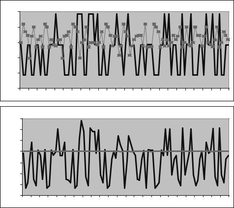
Figure 4.1.A shows 97 simulated values of St+1/St and Ft/St generated from the model. Notice that these two series appear to be negatively correlated. This certainly is not what you would expect to see if uncovered interest parity held. But we know from chapter 1 that market participation of risk-averse agents is potentially a key reason behind the failure of UIP.

Figure 4.1.B shows the simulated values of the predicted forward payo Et(St+1 − Ft)/St and the realized payo (St+1 − Ft)/St. The thing to notice here is that the predicted payo or risk premium seems too small to explain the data. The largest predicted state contingent

(96) risk premium is actually only 0.14 percent on a quarterly basis.

Now we generate 10000 time-series observations from the model and use them to calculate slope coe cient, volatility, and autocorrelation coe cients shown in the row labeled ‘model’ in Table 4.2. As can be seen, the implied volatility of the depreciation and of the realized proÞt

4.5. CALIBRATING THE LUCAS MODEL

131

is much too small. The implied persistence of the depreciation and the forward premium is also too low to be consistent with the data.

The model does predict that the forward rate is a biased predictor of the future spot rate due to the presence of a risk premium. However, the size of the implied risk premium appears to be too small to provide an adequate explanation for the data. We study the forward premium puzzle in greater detail in chapter 6.

132	CHAPTER 4. THE LUCAS MODEL

1.02		A. Depreciation and Forward Premium
1.01
1.00
0.99
0.98
0.97
73	75	77	79	81	83	85	87	89	91	93	95

B. Ex Post Profit and Risk Premium

0.03
0.02
0.01
0.00
-0.01
-0.02
-0.03
-0.04
73	75	77	79	81	83	85	87	89	91	93	95

Figure 4.1: From the Lucas Model. A: Implied gross one-period ahead change in nominal exchange rate St+1/St and current forward premium Ft/St (in boxes). B. Implied ex post forward payo (St+1 − Ft)/St (jagged line) and risk premium Et(St+1 − Ft)/St (smooth line).

4.5. CALIBRATING THE LUCAS MODEL

133

Lucas Model Summary

1.It is a ßexible-price, complete markets, dynamic general equilibrium model with optimizing agents. It is logically consistent and provides the micro-foundations for international asset pricing.

2.The Lucas model provides a framework for pricing assets, including the exchange rate, in an international setting. The exchange rate depends on the same set of fundamental variables as predicted by the monetary model. The empirical predictions of the model will be developed more fully in chapter 6.

3.There is no trading volume for any of the assets. The prices derived in the model are shadow values under which the existing stock of assets are willingly held by the agents.

4.Output is taken to be exogenous so the model not well equipped to explain quantities such as the current account.

5.The Lucas model is designed to help us understand the determination of the prices of assets–exchange rates, bonds, and stocks–that are consistent with equilibrium choices of consumption. Because it is an endowment model, the dynamics of consumption (or alternatively output) are taken exogeneously. This is actually a virtue of the model since a model with production, while perhaps more ‘realistic,’ does not change the underlying asset pricing formulae which are based on the Euler equations for the consumer’s problem but complicates the job by forcing us to write down a model where equilibrium decisions of the Þrm generate not only realistic asset price movements but also realistic output dynamics. It is therefore not necessary or even desirable to introduce production in order to understand equilibrium asset pricing issues.