10.3. INFINITESIMAL MARGINAL INTERVENTION

317

0.03
						s
0.02
0.01
0										f
-0.03	-0.02	-0.02	-0.01	0.00	0.00	0.01	0.01	0.02	0.02	0.03
-0.01	G(f)
-0.02
	s=f
-0.03

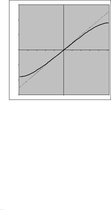
Figure 10.1: Relation between exchange rate and fundamentals under pure ßoat and Krugman interventions

Estimating and Testing the Krugman Model

DeJong [36] estimates the Krugman model by maximum likelihood and by simulated method of moments (SMM) using weekly data from January 1987 to September 1990. He ends his sample in 1990 so that exchange rates a ected by news or expectations about German reuniÞcation, which culminated in the European Monetary System crisis of September 1992, are not included.

We will follow De Jong’s SMM estimation strategy to estimate the basic Krugman model

∆ft	=	η + σut,
Gt	= αη + ft + Aeλ1ft + Beλ2ft ,

¯ iid

where f = −f, the time unit is one day (∆t = 1), and ut N(0, 1). λ1

and λ2 are given in (10.34)-(10.35), and A and B are given in (10.38)

318 CHAPTER 10. TARGET-ZONE MODELS

and (10.39). The observations are daily DM prices of the Belgian franc, French franc, and Dutch guilder from 2/01/87 to 10/31/90. Log exchange rates are normalized by their central parities and multiplied by 100. The parameters to be estimated are (η, α, σ, f¯). SMM is covered in Chapter 2.3.

Denote the simulated observations with a ‘tilde.’ You need to simulated sequences of the fundamentals that are guaranteed to stay within the bands [f, f¯]. You can do this by letting fˆj+1 = f˜j + η + σuj and

setting

fˆ

if fj+1

≥ˆ f

¯

˜

¯

ˆ

¯

≤

≤

fj+1

if

ˆ

fj+1

f

(10.41)

= fj+1

f

f

if

fj+1 ≤ f

for j = 1, . . . , M. The simulated exchange rates are given by

s˜j(η, α, σ, f¯) = f˜j + αη + Aeλ1f˜j

+ Beλ2f˜j ,

(10.42)

the simulated moments by

M Pj=3 ∆s˜j

1

M

∆s˜j

HM [˜s(η, α, σ, f¯)] =

M

j=3

.

M

Pj=3

∆s˜j

1

M

2

1

M

∆s˜j∆s˜j 1

M

jP

1

M

−

3

1

M

M

Pj=3 ∆s˜j∆s˜j 2

P

=3

−

The sample moments are based on the Þrst three moments and the Þrst two autocovariances

				T	P	T
			1				∆st
Ht(s) =				T		t=3
				T	Pt=3 ∆st
				1		tT=3 ∆st2
		1			T	∆st∆st 1
		T			tP
						T	−
			1		T
		5	P		=3		−
		1	Pt=3			∆s ∆s
		T					t t 2

with M = 20T, where T = 978.

The results are given in Table 10.1. As you can see, the estimates are reasonable in magnitude and have the predicted signs, but they are not very precise. The χ2 test of the (one) overidentifying restriction is rejected at very small signiÞcance levels indicating that the data are inconsistent with the model.

5No adjustments were made for weekends or holidays.