(54)

(55)

74 CHAPTER 2. SOME USEFUL TIME-SERIES METHODS

Linear Filters

You can see how a Þlter changes the character of a time series by comparing the spectral density function of the original observations with that of the Þltered data.

Let the original data qt have the Wold moving-average representation, qt = b(L)²t where b(L) = P∞ bjLj and ²t iid with E(²t) = 0

j=0

and Var(²t) = σ²2. The k-th autocovariance is

γk = E(qtqt−k) = E[b(L)²tb(L)²t−k]											bjbj−k ,
= E			∞		bj²t−j	bs²t−s−k = σ²2			∞
						∞
		X				X		jX
		j=0				s=0			=0
and the autocovariance generating function for qt is
g(z) =	γkzk =				∞	σ²2	bjbj−k zk
∞							∞
X					k X		X
−∞					−∞
k=	σ²2				=		j=0				bjzjbj−kz−(j−k)
=			∞		bjbj−k zkzjz−j = σ²2
∞							∞			∞
X			X				k X X
−∞			j=0				=	−∞		j=0
k=
= σ²2		bjzj			bj−kz−(j−k) = σ²2b(z)b(z−1).
∞					∞
X				X
j=0				k=j

But from (2.111), you know that s(ω) = g(2eπiω) . To summarize, these results, the spectral density of qt can be represented as

	s(ω) =		1	g(e−iω) =	1	σ2b(e−iω)b(eiω).	(2.112)
					2π
			2π			²
Let the transformed (Þltered) data be given by q˜t =							a(L)qt where
b(L) =	P						˜
a(L) =	∞	j
	j=−∞ ajL . Then q˜t = a(L)qt = a(L)b(L)²t = b(L)²t, where
˜	a(L)b(L).	Clearly, the autocovariance generating function of

˜ ˜

the Þltered data is g˜(z) = σ²2b(z)b(z−1) = σ²2a(z)b(z)b(z−1)a(z−1) = a(z)a(z−1)g(z), and letting z = e−iω, the spectral density function of

the Þltered data is

s˜(ω) = a(e−iω)a(eiω)s(ω).

(2.113)

2.7. FILTERING

75

The Þlter has the e ect of scaling the spectral density of the original observations by a(e−iω)a(eiω). Depending on the properties of the Þlter, some frequencies will be magniÞed while others are downweighted.

One way to classify Þlters is according to the frequencies that are allowed to pass through and those that are blocked. A high pass Þlter lets through only the high frequency components. A low pass Þlter allows through the trend or growth frequencies. A business cycle pass Þlter allows through frequencies ranging from 6 to 32 quarters. The most popular Þlter used in RBC research is the Hodrick—Prescott Þlter, which we discuss next.

The Hodrick—Prescott Filter

Hodrick and Prescott [76] assume that the original series qt is generated by the sum of a trend component (τt) and a cyclical (ct) component, qt = τt + ct. The trend is a slow-moving low-frequency component and is in general not deterministic. The objective is to construct a Þlter to to get rid of τt from the data. This leaves ct, which is the part of the data to be studied. The problem is that for each observation qt, there are two unknowns (τt and ct). The question is how to identify the separate components?

The cyclical part is just the deviation of the original series from the long-run trend, ct = qt − τt. Suppose your identiÞcation scheme is to minimize the variance of the cyclical part. You would end up setting its variance to 0 which means setting τt = qt. This doesn’t help at all—the trend is just as volatile as the original observations. It therefore makes sense to attach a penalty for making τt too volatile. Do this by minimizing the variance of ct subject to a given amount of prespeciÞed ‘smoothness’ in τt. Since ∆τt is like the Þrst derivative of the trend and ∆2τt is like the second derivative of the trend, one way to get a smoothly evolving trend is to force the Þrst derivative of the trend to evolve smoothly over time by limiting the size of the second derivative. This is what Hodrick and Prescott suggest. Choose a sequence of points {τt} to minimize

T	T−1
X	Xt
(qt − τt)2 + λ	(∆2τt+1)2,	(2.114)
t=1	=1

76 CHAPTER 2. SOME USEFUL TIME-SERIES METHODS

where λ is the penalty attached to the volatility of the trend component. For quarterly data, researchers typically set λ = 1600.33 Noting that ∆2τt+1 = τt+1 − 2τt + τt−1, di erentiate (2.114) with respect to τt and re-arrange the Þrst-order conditions to get the Euler equations

q1 − τ1 = λ[τ3 − 2τ2 + τ1],
q2 − τ2 = λ[τ4 − 4τ3 + 5τ2 − 2τ1],
	.			.
	.			.
	.			.
qt − τt		= λ[τt+2 − 4τt+1 + 6τt − 4τt−1 + τt−2],																t = 3, . . . , T − 2
	.			.
	.			.
	.			.
qT −1 − τT−1 = λ[−2τT + 5τT −1 − 4τT −2 + τT−3],
qT − τT = λ[τT − 2τT −1 + τT −2].
Let c = (c1, . . . , cT )0, q = (q1, . . . , qT )0, and τ = (τ1, . . . , τT )0, and write
the Euler equations in matrix form
									q = (λG + IT )τ,											(2.115)
where the T × T matrix G is given by																					· · ·			0
	2	−5		4				1	· ·0			·
	1		2	1				0			·	· ·0									· · ·			0
	−1		4	−6				4			1													0
	0	−	1	4		−		6			4	1	· · ·								· · ·
									−				0
				−
..				..	.								..	.										..
.																								.
G =																									.
	0													0	1	−		4	6	4		1		0
.																				−
.															0			1	4	6		4		1
.																					−
																			−
..																		0	1	4		5		2
.																							−
	0																		0	−		2		1
																				1
		· · ·															· · ·				−

Get the trend component by τ = (λG+IT )−1q. The cyclical component

follows by subtracting the trend from the original observations

c = q − τ = [IT − (λG + IT )−1]q.

33The following derivation of the Þlter follows Pederson [121].

4λ[1−cos(ω)]2

2.7. FILTERING

77

Properties of the Hodrick—Prescott Filter

For t	= 3, . . . , T − 2, the Euler equations can		be2	written
qt − τt = λu(L)τt, where u(L) = (1 − L)2(1 − L−1)2 =			j=−2 ujLj
with u−2	= u2 = 1, u−1 = u1 = −4, and u0 = 6. We	note for future
			P

reference that ct = qt − τt implies that ct = λu(L)τt.

You’ve already determined that qt = (λu(L) + 1)τt = v(L)τt where v(L) = 1 + λu(L) = 1 + λ(1 − L)2(1 − L−1)2, so it follows that

τt = v(L)−1qt = 1 + λ(1 − Lq)t2(1 − L−1)2 .

v−1(L) is the trend Þlter. Once you compute τt, subtract the result from the data, qt to get ct. This is equivalent to forming ct = δ(L)qt where

	δ(L) = 1	−	v−1(L) =	λ(1 − L)2(1 − L−1)2	.
				1 + λ(1 − L)2(1 − L−1)2

Since (1 − L)2(1 − L−1) = L−2(1 − L)4, the Þlter is equivalent to Þrst applying (1 −L)4 on qt, and then applying λL−2v−1(L) on the result.34 This means the Hodrick-Prescott Þlter can induce stationary into the cyclical component from a process that is I(4).

The spectral density function of the cyclical component is sc(ω) = δ(e−iω)δ(eiω)sq(ω), where

δ(e−iω) =	λ[(1 − e−iω)(1 − eiω)]2	.
	λ[(1 − e−iω)(1 − eiω)]2 + 1

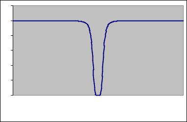
From our trigonometric identities, (1−e−iω)(1−eiω) = 2(1−cos(ω)), it follows that δ(ω) = 4λ[1−cos(ω)]2+1 . Each frequency of the original series

is therefore scaled by	|	δ(ω)	2	=	h	4λ(1−cos(ω))2	2	. This scaling factor is
plotted in Figure 2.4.		|				4λ(1−cos(ω))2+1 i

(56)

(57)

(58)

34This is shown in King and Rebelo (84).

78 CHAPTER 2. SOME USEFUL TIME-SERIES METHODS

1.2
1
0.8
0.6
0.4
0.2
0
3.1	2.8	2.4	2.1	1.7	1.4	1.0	0.7	0.3	0 .0	0 .4	0 .7	1 .1	1 .4	1 .8	2 .1	2 .5	2 .8
- - - - - - - - -
								Frequency

Figure 2.4: Scale factor |δ(ω)|2 for cyclical component in the Hodrick— Prescott Þlter.