Chapter 5

International Real Business

Cycles

In this chapter, we continue our study of models with perfect markets in the absence of nominal rigidities but turn our attention understanding how business cycles originate and how they are propagated and transmitted from one country to another through current account imbalances. For this purpose, we will study real business cycle models. These are stochastic growth models that have been employed to address business cycle ßuctuations. As their name suggests, real business cycle models deal with the real side of the economy. They are Arrow—Debreu models in which there is no role for money and their solution typically focuses on solving the social planner’s problem.

Analytic solutions to the stochastic growth model are available only under special speciÞcations—for example when utility is time-separable and logarithmic and when capital fully depreciates each period. Complications beyond these very simple structures require that the model be solved and evaluated numerically. We will work with durable capital along with the log utility speciÞcation. The resulting models are simple enough for us to retain our intuition for what is going on but complicated enough so that we must solve them using numerical and approximation methods.

Real business cycle researchers evaluate their models using the calibration method, which was outlined in chapter 4.4.4.

137

138 CHAPTER 5. INTERNATIONAL REAL BUSINESS CYCLES

5.1Calibrating the One-Sector Growth Model

We begin simply enough, with the closed economy stochastic growth model with log utility and durable capital. Then we will construct an international real business cycle model by piecing two one-country models together.

Measurement

The job of real business cycle models is to explain business cycles but the data typically contains both trend and cyclical components.1 We will think of a macroeconomic time series such as GDP, as being built up of the two components, yt = yτt + yct, where yτt is the long-run trend component and yct is the cyclical component. Since businesscycle theory is typically not well equipped to explain the trend, the Þrst thing that real business cycle theorists do is to remove the noncyclical components by Þltering the data.

There are many ways to Þlter out the trend component. Two very crude methods are either to work with Þrst-di erenced data or to use least-squares residuals from a linear or quadratic trend. Most real business cycle theorists, however choose to work with Hodrick—Prescott [76] Þltered data. This technique, along with background information on the spectral representation of time-series is covered in chapter 2.

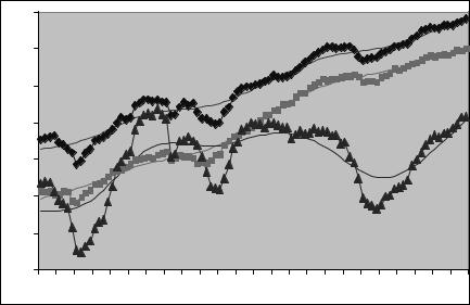
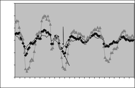
Our measurements are based on quarterly log real output, consumption of nondurables plus services, and gross business Þxed investment in per capita terms for the US from 1973.1 to 1996.4. The output measure is GDP minus government expenditures. The raw data and HodrickPrescott trends are displayed in Figure 5.1. The Hodrick-Prescott cyclical components are displayed in Figure 5.2. Investment is the most volatile of the series and consumption is the smoothest but all three are evidently highly correlated. That is, they display a high degree of ‘co-movement.’

Table 5.1 displays some descriptive statistics of the Þltered (cyclical part) data. Each series displays substantial persistence and a high degree of co-movement with output.

1The data also contains seasonal and irregular components which we will ignore.

5.1. CALIBRATING THE ONE-SECTOR GROWTH MODEL 139

0.2
0.1						GDP
0									Consumption
-0.1
-0.2
-0.3							Investment
-0.4
-0.5
73	75	77	79	81	83	85	87	89	91	93	95

Figure 5.1: US data (symbols) and trend (no symbols) from HodrickPrescott Þlter. Observations are quarterly per capita logarithms of GDP, consumption, and investment from 1973.1 to 1996.4.

The model

We will work with a version of the King, Plosser, and Rebelo [83] model that abstracts from the labor-leisure choice. The consumer has logarithmic period utility deÞned over the single consumption good

u(C) = ln(C). Lifetime utility is P∞ βju(Ct+j), where 0 < β < 1 is

j=0

the subjective discount factor.

The representative Þrm produces output Yt, by combining labor Nt, and capital Kt, according to a Cobb-Douglas production function. Individuals are compelled to provide a Þxed amount of N hours of labor to the Þrm each period. Permanent changes to technology take place through changes in labor productivity, Xt. The number of e ective labor units is NXt. This part of technical change is assumed to evolve exogeneously and deterministically at a gross rate of γ = Xt+1/Xt. A second component that governs technology is a transient stochastic

140 CHAPTER 5. INTERNATIONAL REAL BUSINESS CYCLES

0.15
0.1			Investment
0.05					GDP
0
-0.05
-0.1						Consumption
-0.15
73	75	77	79	81	83	85	87	89	91	93	95

Figure 5.2: Hodrick-Prescott Þltered cyclical observations.

shock, At. The production function is

Yt = AtKtα(NXt)1−α.

α is capital’s share. Most estimates for the US place 0.33 ≤ α ≤ 0.40. Output can be consumed or saved. Savings (or investment It) are used to replace worn capital and to augment the current capital stock.

Capital depreciates at a rate δ and evolves according to

Kt+1 = It + (1 − δ)Kt.

There is no government and no foreign sector. There are also no market imperfections so we can work with Þctitious social planner’s problem as we did with the Lucas model.

Problem 1. The social planner wants to maximize

∞
jX
Et βjU(Ct+j),	(5.1)
=0

5.1. CALIBRATING THE ONE-SECTOR GROWTH MODEL 141

Table 5.1: Closed-Economy Measurements

						Std.				Autocorrelations
						Dev.			1		2		3		4		6
			yt			0.022		0.86		0.66		0.46		0.27		0.02
			ct			0.013		0.85		0.72		0.57		0.38		0.14
			it			0.056		0.89		0.73		0.56		0.40		0.08
							Cross correlation with yt−k at k
				6			4		1		0		-1		-4		-6
	ct			0.09			0.20		0.72		0.87		0.87		0.46		0.14
	it			0.01			0.43		0.91		0.94		0.81		0.20		0.10

Notes: All variables are logarithms of real per capita data for the US from 1973.1 to 1996.4 and have been passed through the Hodrick—Prescott Þlter with λ = 1600. yt is gross domestic product less government spending, ct is consumption of nondurables plus services, and it is gross business Þxed investment. Source: International Financial Statistics.

subject to Yt = AtKα(NXt)1−α,	(5.2)
t
Kt+1 = It + (1 − δ)Kt,	(5.3)
Yt = Ct + It,	(5.4)
U(C) = ln(C).	(5.5)

The model allows for one normalization so you can set N = 1.

In the steady state, you will want the economy to evolve along a balanced growth path in which all quantities except for N grow at the same gross rate

γ = Xt+1 = Yt+1 = Ct+1 = It+1 = Kt+1 .
Xt	Yt	Ct	It	Kt

The steady state is reasonably straightforward to obtain. However, if capital lasts more than one period, δ < 1, the dynamics of the model must be solved by approximation methods. We’ll Þrst solve for the steady state and then take a linear approximation of the model around its steady state. The exogenous growth factor γ gives the model a

142 CHAPTER 5. INTERNATIONAL REAL BUSINESS CYCLES

moving steady state which is inconvenient. To Þx this, you can Þrst transform the model to get a Þxed steady state by normalizing all the variables by labor e ciency units. Let lower case letters denote these normalized values

yt

=

Yt

, kt =

Kt

, it =

It

, ct =

Ct

.

Xt

Xt

Xt

Xt

Dividing (5.2) by Xt gives yt

= Atktα.

Dividing (5.3) by Xt gives

γkt+1 = it + (1 − δ)kt. To normalize lifetime utility (5.1), note that

P ln(Xt)/(1 − β) P

∞

−

∞

P

∞

jβj

∞

j

ln Xt+j

j

j

= ln(X )/(1

−

β) + ln(γ)

(ch.5-1)

j=0 β

=

j=0

β

ln(γ

Xt)

2

<

t

.

j=0

=

+ ln(γ)β/(1

β)

Using this fact,

adding

Ωt + Et j=0

β UPt+j

j

t

P

t

and subtracting

∞

∞

j

U(Ct+j) =

j=0 β

ln(Xt+j) to (5.1) gives Et j=0

β

β ln(γ)/P −

t

∞

j

(c

) where U(c) = ln(c) and Ω = ln(X )/(1

−

β) +

(1

2

β)

. Since Ω is exogenous, we can ignore it when solving

the planner’s problem. We will call the transformed problem, problem 2. This is the one we will solve.

Problem 2. It will be useful to use the notation f(At, kt) = Atkα. Since Ω is a constant, the social planner’s growth problem normalized by labor e ciency units is to maximize

	∞
	jX
Et	βjU(ct+j),	(5.6)
	=0
subject to yt	= f(At, kt) = Atkα,	(5.7)
	t
γkt+1 = it + (1 − δ)kt,		(5.8)
yt = ct + it,		(5.9)
U(c) = ln(c).		(5.10)

It will be useful to compactify the notation. Let λt = (kt+1, kt, At)0 and combine the constraints (5.7)—(5.9) to form the consolidated budget constraint

ct = g(λt) =	f(At, kt) − γkt+1 + (1 − δ)kt
=	Atktα − γkt+1 + (1 − δ)kt.	(5.11)

Under Cobb-Douglas production and log utility, you have

αy y 1 −1 fk = k , fkk = α(α − 1)k2 , uc = c, ucc = c2 .

5.1. CALIBRATING THE ONE-SECTOR GROWTH MODEL 143

Letting gj = ∂ct/∂λjt be the partial derivative of g(λt) with respect to the j−th element of λt and gij = ∂2ct/(∂λit∂λjt) be the second cross-partial derivative, for future reference you have

g1 = −γ,

g2 = fk(A, k) + (1 − δ), g3 = y/A,

g11 = g12 = g21 = g13 = g31 = g33 = 0,

g22 = fkk(A, k),

g23 = g32 = αkα−1.

Now substitute (5.11) into (5.6) to transform the constrained optimization problem into an unconstrained problem. You want to maxi-

mize
∞
jX
Et βju[g(λt+j)],	(5.12)
=0

where g(λt) is given in (5.11). At date t, kt is pre-determined and the only choice variable is it and choosing it is equivalent to choosing kt+1. The Þrst-order conditions for all t are

−γuc(ct) + βEtuc(ct+1)[fk(At+1, kt+1) + (1 − δ)] = 0.

(5.13)

Notice that ct must obey the consolidated budget constraint (5.11). It follows that (5.13) is a nonlinear stochastic di erence equation in kt. Analytic solutions to such equations are not easy to obtain so we resort to approximation methods.

The Steady State

We will compute the approximate solution around the model’s steady state. In order to do that we need Þrst to Þnd the steady state. Denote steady state values of output, consumption, investment and capital y, c, i, k without the time subscript and let the steady state value of A = 1.

Since fk = αkα−1 = α(y/k), (5.13) becomes γ = β[α(y/k) + (1 − δ)] from which we obtain the steady state output to capital ratio

144 CHAPTER 5. INTERNATIONAL REAL BUSINESS CYCLES

y/k = (γ/β + δ −1)/α. Now divide the production function (5.7) by k and re-arrange to get k = (y/k)1/(α−1) = [(γ/β + δ − 1)/α]1/(α−1). Now that we know k, we can get y. From the accumulation equation (5.8), we have i/k = γ + δ −1, and in turn, c/k = y/k −i/k. Again, given k, we can solve for c. To summarize, in the steady state we have

y/k	=	(γ/β + δ − 1)/α,	(5.14)
i/k	=	γ + δ − 1,	(5.15)
c/k	=	y/k − i/k,	(5.16)
k	=	(y/k)1/(α−1).	(5.17)

Calibrating the Model
Each	time period corresponds to a	quarter. We set α	= 0.33,
β =	0.99, δ = 0.10, γ = 1.0038.2	The transient technology shock
evolves according to the Þrst-order autoregression
	At = (1 − ρ) + ρAt−1 + ²t,		(5.18)
	iid
where ρ = 0.93, and ²t N(0, 0.0102242).

Approximate Solution Near the Steady State.

Many methods have been applied to solve real business cycle models. One option for solving the model is to take a Þrst—order Taylor expansion of the nonlinear Þrst—order condition (5.13) in the neighborhood around the steady state.3. This yields the second—order stochastic di erence equation in kt − k

a0 +a1(kt+2 −k)+a2(kt+1 −k)+a3(kt −k)+a4(At+1 −1)+a5(At −1) = 0, (5.19)

2This is the depreciation rate used by Backus et. al. [5]. Cooley and Prescott [33] recommend δ = 0.048. γ is the value used by Cooley and Prescott and King et. al..

3This is the method of King, Plosser, and Rebelo [83]

5.1. CALIBRATING THE ONE-SECTOR GROWTH MODEL 145

where a0	= Ucg1 + βUcg2 = 0,
a1 = βUccg1g2,
a2 = Uccg12 + βUccg22 + βUcg22,
a3	= Uccg1g2,
a4	= βUcg32 + βUccg2g3,
a5	= Uccg1g3.

The derivatives are evaluated at steady state values.

A second but equivalent option is to take a second—order Taylor approximation to the objective function around the steady state and to solve the resulting quadratic optimization problem. The second option is equivalent to the Þrst because it yields linear Þrst—order conditions around the steady state. To pursue the second option, recall that λt = (kt+1, kt, At)0. Write the period utility function in the unconstrained optimization problem as

R(λt) = U[g(λt)].

(5.20)

Let Rj = ∂R(λt)/∂λjt be the partial derivative of R(λt) with respect to the j−th element of λt and Rij = ∂2R(λt)/(∂λit∂λjt) be the second cross-partial derivative. Since Rij = Rji the relevant derivatives are,

R1 = Ucg1,

R2 = Ucg2,

R3 = Ucg3,

R11 = Uccg12,

R22 = Uccg22, +Ucg22

R33 = Uccg32,

R12 = Uccg1g2,

R13 = Uccg1g3,

R23 = Uccg2g3 + Ucg23.

The second-order Taylor expansion of the period utility function is

R(λt) = R(λ) + R1(kt+1 − k) + R2(kt − k) + R3(At − A) +	1	R11(kt+1	− k)2
	2

146 CHAPTER 5. INTERNATIONAL REAL BUSINESS CYCLES

+12R22(kt − k)2 + 12R33(At − A)2 + R12(kt+1 − k)(kt − k) +R13(kt+1 − k)(At − A) + R23(kt − k)(At − A).

Suppose we let q = (R1, R2, R3)0 be the 3 × 1 row vector of partial derivatives (the gradient) of R, and Q be the 3 × 3 matrix of second partial derivatives (the Hessian) multiplied by 1/2 where Qij = Rij/2. Then the approximate period utility function can be compactly written in matrix form as

	R(λt) = R(λ) + [q + (λt − λ)0Q](λt − λ).			(5.21)
The problem is now to maximize
	∞
	jX
	E βjR(λ		).	(5.22)
	t	t+j
	=0
The Þrst order conditions are for all t
0 = (βR2 + R1) + βR12(kt+2 − k) + (R11 + βR22)(kt+1 − k) + R12(kt − k)
	+βR23(At+1 − 1) + R13(At − 1).			(5.23)
If	you compare (5.23) to (5.19), you’ll		see that a0 =	βR2 + R1,
a1	= βR12, a2 = R11 + βR22, a3	= R12, a4 = βR23, a5 = R13. This
veriÞes that the two approaches are indeed equivalent.

Now to solve the linearized Þrst-order conditions, work with (5.19). Since the data that we want to explain are in logarithms, you can convert the Þrst-order conditions into near logarithmic form. Let a˜i = kai for i = 1, 2, 3, and let a “hat” denote the approximate log

ˆ

di erence from the steady state so that kt = (kt − k)/k ' ln(kt/k)

ˆ

and At = At − 1 (since the steady state value of A = 1). Now let b1 = −a˜2/a˜1, b2 = −a˜3/a˜1, b3 = −a4/a˜1, and b4 = −a4/a˜1.

The second—order stochastic di erence equation (5.19) can be written as

2	ˆ	= Wt,	(5.24)
(1 − b1L − b2L )kt+1
where
ˆ		ˆ
Wt = b3At+1	+ b4At.

5.1. CALIBRATING THE ONE-SECTOR GROWTH MODEL 147

The roots of the polynomial (1 − b1z − b2z2) = (1 − ω1L)(1 − ω2L) satisfy b1 = ω1 + ω2 and b2 = −ω1ω2. Using the quadratic formula

and evaluating at the parameter values that we used to calibrate the

q

model, the roots are, z1 = (1/ω1) = [−b1 − b12			+ 4b2]/(2b2) ' 1.23, and
q

z2 = (1/ω2) = [−b1 + b21 + 4b2]/(2b2) ' 0.81. There is a stable root, |z1| > 1 which lies outside the unit circle, and an unstable root, |z2| < 1

which lies inside the unit circle. The presence of an unstable root means that the solution is a saddle path. If you try to simulate (5.24) directly, the capital stock will diverge.

To solve the di erence equation, exploit the certainty equivalence property of quadratic optimization problems. That is, you Þrst get the perfect foresight solution to the problem by solving the stable root backwards and the unstable root forwards. Then, replace future random variables with their expected values conditional upon the time-t information set. Begin by rewriting (5.24) as

Wt =

ˆ

(1 − ω1L)(1 − ω2L)kt+1

ˆ

=

−1

L

−1

)(1 −

(−ω2L)(−ω2

ω2L)(1 − ω1L)kt+1

=

−1

L

−1

ˆ

(−ω2L)(1 − ω2

)(1 − ω1L)kt+1,

and rearrange to get

(1

−

ω

L)kˆ

=

−ω2−1L−1

W

1

t+1

1

−

ω−1L−1 t

12

∞

1

¶

j

= −µ

ω2 L−1¶ j=0

µω2

Wt+j

X

∞

1

j

X

µ

¶ Wt+j.

=

−j=1

ω2

(5.25)

The autoregressive speciÞcation (5.18) implies the prediction formulae

ˆ

ˆ

j ˆ

EtWt+j = b3EtAt+j+1 + b4EtAt+j

= [b3ρ + b4]ρ At.

Use this forecasting rule in (5.25) to get

¶

= "ω2

ρ#

j=1

µω2

¶ EtWt+j = [b3ρ + b4]Aˆt

j=1

µω2

(b3ρ + b4)Aˆt.

∞

1

j

∞

ρ

j

ρ

X

X

−

148 CHAPTER 5. INTERNATIONAL REAL BUSINESS CYCLES

It follows that the solution for the capital stock is

"#

ˆ	ˆ	ρ	ˆ
kt+1	= ω1kt −	ω2 − ρ	[b3ρ + b4]At.	(5.26)

To recover yˆt, note that the Þrst-order expansion of the produc-

ˆ	ˆ	= 1, and
tion function gives yt = f(A, k) + fAAt + fkkkt, where fA
ˆ ˆ	ˆ

fk = (αy)/k. Rearrangement gives yˆt = At + kt. To recover it, subtract

the steady state value γk = i + (1 −δ)k from (5.8) and rearrange to get

ˆ	ˆ	ˆ	ˆ
it = (k/i)[γkt+1		−(1−δ)kt]. Finally, get cˆt = yˆt −it from the adding-up

constraint (5.9). The log levels of the variables can be recovered by

ln(Yt) = yˆt + ln(Xt) + ln(y), ln(Ct) = cˆt + ln(Xt) + ln(c),

ˆ

ln(It) = it + ln(Xt) + ln(i), ln(Xt) = ln(X0) + t ln(γ).

Simulating the Model

We’ll use the calibrated model to generate 96 time-series observations corresponding to the number of observations in the data. From these pseudo-observations, recover the implied log-levels and pass them through the Hodrick-Prescott Þlter. The steady state values are

y = 1.717, k = 5.147, c = 1.201, i/k = 0.10.

Plots of the Þltered log income, consumption, and investment observations are given in Figure 5.3 and the associated descriptive statistics are given in Table 5.2. The autoregressive coe cient and the error variance of the technology shock were selected to match the volatility of output exactly. From the Þgure, you can see that both consumption and investment exhibit high co-movements with output, and all three series display persistence. However from Table 5.2 the implied investment series is seen to be more volatile than output but is less volatile than that found in the data. Consumption implied by the model is more volatile than output, which is counterfactual.