6.3. TESTING EULER EQUATIONS

177

This is why market e ciency does not mean that the exchange rate must follow a random walk or that uncovered interest parity must hold. The Lucas model predicts that in equilibrium, it is the marginal utility of the forward contract payo that is unpredictable and that deviations from UIP can emerge as compensation for risk bearing.

6.3Testing Euler Equations

Using the methods of Hansen and Singleton [73], Mark [100] estimated and tested the Euler equation restrictions using 1-month forward exchange rates. Modjtahedi [106] goes a step further and tests implied Euler equation restrictions across the entire a term structure available for forward rates (1, 3, 6, and 12 months). The strategy is to estimate the coe cient of relative risk aversion γ and test the orthogonality conditions implied by the Euler equation (6.11) using GMM.

Here, we use non-overlapping quarterly observations on dollar rates of the pound, deutschemark, and yen from 1973.1 to 1997.1 and revisit Mark’s analysis. To write the problem compactly, let rt+1 be the 3 × 1 forward foreign exchange payo vector

			(F1t−S1t+1)
			(S1t)
			(F2t S2t+1)
rt+1	=		−			,
			(S2t)
			(F3t S3t+1)
			−
			(S3t)
and let the 3 × 1 vector wt+1 be
wt+1 = µtm+1rt+1,						(6.17)

where µmt+1 is the US representative investor’s intertemporal marginal rate of substitution of money under CRRA utility, u(C) = C1−γ/(1−γ).

Using the notation developed here to rewrite the Euler equations (6.11) you get

E[wt+1|It] = 0.

(6.18)

Divide both sides by β so that you only need to estimate γ. (6.18) says that wt+1 is uncorrelated with any time-t information. Let zt be a k−dimensional vector of time-t ‘instrumental variables,’ available

178CHAPTER 6. FOREIGN EXCHANGE MARKET EFFICIENCY

to you, the econometrician. Then (6.18) implies the following 3 × k estimable and testable equations4

E[wt+1 zt] = E[(µtm+1rt+1) zt] = 0.

(6.19)

Now the question is what to choose for zt? It is not a good idea to use too many variables because the estimation problem will become intractable and the small sample properties of the GMM estimator will su er. A good candidate is the forward premium since we know that it is directly relevant to the problem at hand. Furthermore, it is not necessary to use all the possible orthogonality conditions. To reduce the dimensionality of the estimation problem further, for each currency i, let

zit = "	1	#
	(Fit−Sit)
	Sit

be a vector of instrumental variables consisting of the constant 1, and the normalized forward premium. Estimating γ from the system of six equations

E		w1t+1z1t		,	(6.20)
		w2t+1z2t
	w3t+1z3t

gives γˆ = 48.66 with asymptotic standard error of 79.36. The coefÞcient of relative risk aversion is uncomfortably large and imprecisely estimated. However, the test of the Þve overidentifying restrictions gives a chi-square statistic of 7.20 (p-value=0.206) does not reject at standard levels of signiÞcance.

Why does the data force γˆ to be so big? We can get some intuition by recasting the problem as a regression. Suppose you look at just

one currency. If (	Ct	,	Pt	, Ft−St+1 ) are jointly lognormally distributed
			Pt+1
	Ct+1			St

then wt+1 is also lognormal.5						Taking logs, of both sides of (6.17), you
							a11	a12
	denotes the Kronecker product. Let
4							A = µ a21	a22 ¶ and B be any n × k
matrix. Then A			B =	a11B a12B
				µ a21B		a22B ¶.
5
	A random variable X is said to be lognormally distributed if ln(X) is normally

distributed.

rte+1

Pt

(Ft−St+1

6.3. TESTING EULER EQUATIONS								179
get		¶	+ ln Ã		! = −γ ln	Ã		! + ln wt+1.
ln	Ft − St+1			Pt			Ct
	S			P			C
µ	t			t+1			t+1

ln(Ct/Ct+1) is correlated with ln wt+1 so you don’t get consistent estimates with OLS—but you do get consistency with instrumental variables and this is what GMM does. However, the regression analogy tells us that the large estimate of γ and its large standard error can be attributed to high variability in the excess return combined with low variability in consumption growth. The di culty that the Lucas model under CRRA utility to explain the data with small values of γ is not conÞned to the foreign exchange market. The corresponding di - culty for the model to simultaneously explain historical stock and bond returns is what Mehra and Prescott [105] call the ‘equity premium puzzle’.

Volatility Bounds

Hansen and Jagannathan [72] propose a framework to evaluate the extent to which the Euler equations from representative agent asset pricing models satisfy volatility restrictions on the intertemporal marginal rate of substitution.

We will Þrst derive a lower bound on the volatility of the intertemporal marginal rate of substitution predicted by the Euler equations of the intertemporal asset pricing model. Let rt+1 be an N-dimensional vector of holding period returns from t to t+1 available to the agent, and µt+1 = βu0(Ct+1)/u0(Ct) be the intertemporal marginal rate of substitution.

We need to write the Euler equations in returns form. For equities, they take the form 1 = Et(µt+1rte+1) where rte+1 is the gross return.6 It reads—an asset with expected payo Et(µt+1rte+1) costs one unit of the consumption good. An analogous returns form of the Euler equation holds for bonds. In the case of forward foreign exchange contracts, there is no investment required in the current period so the returns form for the Euler equation is 0 = Etµt+1 ) . Thus, the returns form of

6Take the equity Euler equation (4.12)) and = (et+1 + xt+1)/et to get the expression in

divide both sides by etu1,t+1. Let the text.

180CHAPTER 6. FOREIGN EXCHANGE MARKET EFFICIENCY

the Euler equations for asset pricing can generically be represented as

						v = Et(µt+1rt+1),				(6.21)
	where v is a vector of constants whose i − th element vi = 1 if asset i
	is a stock or bond, and vi = 0 if asset i is a forward foreign exchange
	contract.
		Taking the unconditional expectation on both sides of (6.21) and
	using the law of iterated expectations gives
						v = E(µt+1rt+1).				(6.22)
(112)	Let	θµ ≡ E(µt),				σµ2 ≡	E(µt − θµ)2, θr ≡			E(rt), and
	Σr	≡ E(rt − θr)(rt − θr)0. Project (µt − θµ) onto (rt − θr) to obtain
					(µt − θµ) = (rt − θr)0			β	µ + ut,	(6.23)
	where		β	µ is a vector of least squares projection coe cients, ut is the
	least squares projection error and
					β	µ = Σr−1E(rt − θr)(µt − θµ).				(6.24)
	Furthermore, you know that
				E(rt		− θr)(µt	− θµ) = E(rtµt) −θrθµ,			(6.25)
							| {z }

v

where E(rtµt) = v comes from the returns form of the Euler equations. Upon substituting (6.25) into (6.24), we get, βµ = Σ−r 1(v − θrθµ).

Computing the variance of the intertemporal marginal rate of substitution gives

σµ2 = E(µt − θµ)2

= E(µt − θµ)0(µt − θµ)

= E[(rt − θr)0

β

µ + ut]0[(rt − θr)0

β

µ + ut]

= E[

β

µ0 (rt − θr)(rt − θr)0

β

µ] + σu2 +

β

µ0 E(rt − θr)ut + Eut(rt − θr)0βµ

0 −1 −1

|

}

2

({z

a)

= E(µtrt − θµθr) Σr ΣrΣr E(µtrt − θµθr) + σu

= (v − θµθr)0Σr−1(v − θµθr) + σu2.

(6.26)

i1/2

6.3. TESTING EULER EQUATIONS

181

The term labeled (a) above is zero because ut is the least-squares projection error and is by construction orthogonal to rt. Since σu2 ≥ 0, the volatility or standard deviation of the intertemporal marginal rate of substitution must lie above σr where

q

σµ ≥ σr ≡ (v − θµθr)0Σ−r 1(v − θµθr). (6.27)

The right side of (6.27) is the lower bound on the volatility of the intertemporal marginal rate of substitution. If the assets are all equities or bonds v is a vector of ones and the volatility bound is a parabola in (θµ, σµ) space. If the assets are all forward foreign exchange contracts, v is a vector of zeros and the lower volatility bound is a ray from the

origin

h

σr = θµ θ0rΣ−r 1θr . (6.28)

How does one construct and use the volatility bound in practice? First determine v and calculate θr and Σr from asset price data. Then using (6.28) you trace out σr as a function of θµ. Next, for a given functional form of the utility function, use consumption data to calculate the volatility of the intertemporal marginal rate of substitution, σµ. Compare this estimate to the volatility bound and determine whether the bound is satisÞed.

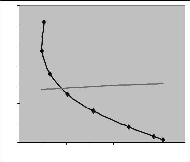
When we do this using quarterly US consumption and CPI data

and dollar exchange rates for the pound, deutschemark, and yen from

q

1973.1 to 1997.1, we get θ0rΣ−1θr = 0.309. Now let the utility function (113) be CRRA with relative risk aversion coe cient γ. As we vary γ, we generate the entries in the following table.

γ	θµ	σµ	σr
2	0.982	0.015	0.303
4	0.974	0.031	0.301
10	0.953	0.078	0.294
20	0.923	0.159	0.285
30	0.901	0.248	0.278
40	0.886	0.349	0.273
50	0.879	0.469	0.272
60	0.881	0.615	0.272

182CHAPTER 6. FOREIGN EXCHANGE MARKET EFFICIENCY

You can see that σµ < σr for values of γ below 30. This means (115) that exchange rate payo s are too volatile relative to the fundamentals

(the intertemporal marginal rate of substitution) over this range of γ. Note how the GMM estimate of γ = 48 obtained earlier in this chapter is consistent with this result. In order to explain the data, the Lucas model with CRRA utility requires people to be very risk averse. Many people feel that the degree of risk aversion associated with γ = 48 is unrealistically high and would rule out many observed risky gambles undertaken by economic agents.

	0.7
	0.6		C =60
			IMRS
	0.5		C =5 0
V o la tility	0.4		C =4 0			Lower Volatility Bound
	0.3
	0.2		C =3 0	C =2 0
	0.1					C =1 0	C =4
								=2
							C
	0
	0.86	0.88	0.9	0.92 Mean	0.94	0.96	0.98	1

Figure 6.2: Mean and volatility estimates of the intertemporal marginal rate of substitution (IMRS) with β = 0.99 and alternative values of γ under constant relative risk aversion utility and lower bound implied by forward exchange payo s of the pound, deutschemark, and yen, 1973.1 to 1997.1.

The mean and volatility of the intertemporal marginal rate of substitution (θµ, σµ) for alternative values of γ and the lower volatility bound

(116) (σr = 0.309θµ) implied by the data are illustrated in Figure 6.2.7