Temporal Resolution

The number of real-time images produced per minute is referred to as the frame rate and is dependent upon the PRF. The faster the frame rate, the faster the pulse repetition frequency (PRF). Faster frame rates produce better temporal resolution (resolution with respect to time). Logically, rapidly moving structures require fast frame rates in order to prevent slow motion or freeze frame images of cardiac motion.

Temporal Resolution

Dependent upon frame rate

Reduce sector width in order to improve the frame rate

Reduce image depth

Sector transducers that emit multiple pulses with varying focal zones per scan line must wait until all sound has returned before generating the next set of pulses otherwise range or depth ambiguity results. In doing so the frame rate and temporal resolution of the generated two-dimensional image is reduced. Interrogation of deep structures also requires a slower frame rate and less temporal resolution is possible. It is possible to increase PRF in both of these settings by reducing sector width and/or image depth since less time is required before the next frame can be produced.

Doppler Physics

Doppler has dramatically increased the diagnostic capabilities of cardiac ultrasound. This modality allows detection and analysis of moving blood cells or myocardium. It tells us about the direction, velocity, character, and timing of blood flow or muscle motion. The hemodynamic information provided by Doppler echocardiography allows definitive diagnosis in most cardiac examinations.

Doppler Ultrasound

Allows detection and analysis of moving blood cells or myocardium and provides hemodynamic information about:

Direction

Velocity

Character

Timing

Four types of Doppler used during an echocardiographic exam will be discussed in this text: pulsedwave (PW) Doppler, continuous-wave (CW) Doppler, color-flow (CF) Doppler, and tissue Doppler imaging (TDI). Pulsed-wave Doppler is site specific. In other words it can be directed and set to sample flow at very specific places within the heart. It is, however, limited in its capacity to detect higher frequency (velocity) shifts. Continuous-wave Doppler has the ability to detect high frequency shifts and therefore can record high-flow velocities with virtually no limits. As you will see, since sound is continuously transmitted and received in CW Doppler, it is not possible to select and interrogate at specific depths within the heart. Although this may sound like a disadvantage, the information provided by CW Doppler is very valuable. Color-flow Doppler is a form of pulsed-wave Doppler. Frequency shifts are encoded with varying hues and intensities of color. Flow information is very vivid, and detection of abnormal flow is easier with color-flow Doppler although quantitative

information is limited. Tissue Doppler imaging uses pulsed-wave Doppler to interrogate myocardial motion and velocities. It is used to assess both systolic and diastolic myocardial function. These various forms of Doppler ultrasound and the factors that influence them are explained and discussed in the following sections.

Pulsed-Wave Doppler

Allows flow to be examined at very specific sites.

It is limited in the maximum velocity that it can accurately record.

Continuous-Wave Doppler

There is no limit to the maximum velocity it can record.

It is not site specific; blood cells are examined all along the sound beam.

Color-Flow Doppler

This is a form of pulsed-wave Doppler.

It color codes the various velocities and directions of flow.

Tissue-Doppler Imaging

This is a form of pulsed-wave Doppler.

It records myocardial velocity.

It is used to assess systolic and diastolic function and synchronicity.

The Doppler Shift

Christian Johann Doppler (1803–1853), an Austrian physicist and mathematician, was the first to describe the Doppler effect. He found that all types of waves (light, sound, etc.) change in wavelength when there is a change in position between the source of the wave and the receiver of the wave. Using sound, if you were moving toward a sound source, the pitch or frequency of that sound would increase, and if you were moving away from that sound source, the frequency would decrease. The change in frequency between sound that is transmitted and sound that is received is the Doppler shift.

The Doppler Shift

There is a change in wavelength (pitch and frequency) when there is a change in position between the sound source and the reflecting structure (blood cells in this case).

When the source and the reflecting surface are both stationary, the transmitted (incident) and reflected wavelengths are equal (Figure 1.17). When the reflecting structure is moving toward the source, sound waves are encountered more often, resulting in an increased number of waves (↑ frequency) being reflected back toward the source. When the reflecting structure is moving away from the source, they travel ahead of the transmitted wave front and sound waves are encountered less frequently resulting a decreased number of sound waves (↓ frequency) reflected back to the source.

Cells moving toward the transducer reflect an increased number of sound waves, and so the received frequency is greater than the transmitted frequency. This is a positive frequency shift.

Cells moving away from the transducer reflect fewer sound waves, and the received frequency is less than the transmitted frequency. This is a negative frequency shift.

Figure 1.17 The change in frequency between sound that is sent out and sound that is reflected is called the Doppler shift. (A) Sound reflected from stationary blood cells will have the same frequency as the transmitted sound. (B) Reflected sound encounters the transmitted wave front less often and a decrease in frequency is perceived when blood cells move away from the transducer. (C) Sound reflected from blood cells moving toward the transducer will have a higher frequency than what was sent out because the reflected waves encounter the incident waves more often.

Everyday examples of Doppler shifts include any loud sound moving toward or away from you such as sirens, trains, marching bands, etc. The sound of a siren as it approaches you will increase in pitch (frequency increases) and then as it passes you, the pitch will decrease (frequency decreases). Doppler radar uses this principle when policemen determine the speed of your car, since, as you will see, the frequency shift is used to determine velocity. Doppler radar is also used in forecasting weather. The Doppler shift as we utilize it in diagnostic ultrasound is the difference in frequency transmitted by the transducer and received frequency reflected from blood cells.

The Doppler Tracing

The Doppler-derived frequency shift (fd) is equal to reflected frequency minus transmitted frequency, therefore, objects moving toward the source result in positive frequency shifts while objects moving away from the source result in negative frequency shifts. The site (gate) for Doppler flow interrogation is selected by the examiner and is represented on the Doppler display as a line (baseline). Positive frequency shifts (flow moving toward the transducer) produce waveforms up from the baseline while negative frequency shifts (flow moving away from the transducer) produce downward deflections on the Doppler tracing (Figure 1.18). These images are called spectral tracings. Velocity scale is displayed along the side of the spectral image. The velocity range is split between the positive and the negative directions of flow. When the baseline is located in the middle of the spectral

display, the total velocity range is displayed equally above and below the baseline (Figure 1.19). When the baseline is moved all the way to the top of the image, the entire velocity range is allocated to downward flow. When it is moved to the bottom of the image, the entire velocity range is allocated to upward flow.

Figure 1.18 The baseline in pulsed-wave Doppler represents the sampling gate. Flow moving toward the transducer creates a positive frequency shift, and velocity will be plotted above the baseline. (A) Mitral valve flow in this apical five-chamber view is toward the transducer and its flow profile is seen above the baseline. (B) Aortic flow, moving away from the transducer in this apical five-chamber view, creates a negative frequency shift, and its flow profile is shown below the baseline.

Figure 1.19 (A) When the baseline is positioned in the middle of the spectral display, the velocity range is displayed equally above (1.0 m/sec) and below the baseline (1.0 m/sec). (B) Moving the baseline to the top of the spectral display allocates all of the velocity range (2.0 m/sec) below the baseline.

Pulsed-Wave Doppler

Pulsing the sound waves allows a transducer to act as a receiver for the signal only during the time interval specified by a sample depth. With pulsed-wave Doppler the transducer will record frequency shifts only during the time interval dictated by the depth of the sample site ignoring all other returning echoes (Figure 1.20). New sound waves will not be transmitted until the transducer has received the echoes from the previous burst. The ability to measure velocity within a small cell at a specified depth along the ultrasound beam is referred to as range resolution, and the site at which sampling is set to occur is referred to as the gate. The gate is manually set by the examiner while watching a twodimensional image.

Figure 1.20 Frequency shifts are recorded only during the time interval indicated by the depth of the sample gate. Deeper gates require more time. (A) A gate depth of 13 cm requires 169 μ/sec while a gate of 10 cm (B) requires only 130 μ/sec for sound to return to the transducer. Lower pulse repetition frequency is required for deeper structures.

Continuous-Wave Doppler

Continuous-wave (CW) Doppler, as the name implies, continuously sends out sound and continuously receives sound. It is not possible to range gate CW Doppler because the transducer has no way of detecting the depth of the reflected signal. CW Doppler detects frequency shifts all along the ultrasound beam with no range resolution. CW Doppler is steered in one of two ways. Imaging CW systems use a cursor representing the Doppler sound beam. The cursor is placed over the twodimensional image and frequency shifts are calculated all along the beam. Non-imaging CW systems use a dedicated CW probe without the luxury of a two-dimensional image. These systems require recognition of characteristic flow profiles.

Velocities along the beam vary, and a full spectrum of frequency shifts is detected with CW Doppler. When CW Doppler is used properly, the highest velocities along the line of interrogation are recorded (Figure 1.21). The highest flow velocities are generally what is of interest and diagnostically important. Lower velocity flows found along the Doppler line of interrogation are hidden within the higher flow profiles. Flow patterns for the various valves and vessels in the heart are very characteristic and usually are easily identified with both PW and CW Doppler.

Figure 1.21 Continuous-wave Doppler detects frequency shifts all along the Doppler sound beam. All velocities are recorded. (A) The highest velocity during systole is flow out the aorta; lesser negative velocities during this time period are recorded but hidden within the aortic flow profile. (B) The CW sound beam also records flow during diastole near the apex of the heart.

The Doppler Equation

Doppler ultrasound can determine blood cell velocity within the heart or in peripheral vessels based upon the Doppler shift. Blood cell velocity (V) is determined using the following formula:

Equation 1.3

Equation 1.3 shows that V is equal to the speed of sound in tissues (C) times the frequency shift (fd) in kHz, divided by the transmitting frequency of the transducer, fo (2.5, 3.5, 5.0, etc.), times the cosine of θ, where θ is equal to the intercept angle of the ultrasound beam with respect to the blood flow.

The speed of sound in tissues is a constant (1,540 m/sec), leaving the interrogation angle, θ, and transducer frequency as variables that can be controlled. Let’s consider these two variables and how they affect the way a Doppler exam should be conducted and interpreted.

Velocity Measurement

Accurate measurements are affected by:

Transducer frequency

Intercept angle

Angle of Interrogation

An important part of the Doppler equation is the cosine of the intercept angle. The closer to parallel the transmitted wave is with the direction of blood flow being interrogated, the more accurate the velocity measurement (Figure 1.22).

Figure 1.22 Frequency shifts are directly dependent upon the cosine of the interrogation angle (θ). (A) The closer to parallel the transmitted Doppler signal is to blood flow the more accurate the velocity will be since the cosine of 0° is one. (B) As the intercept angle, θ, deviates from zero, velocity will be underestimated.

When the Doppler equation is changed to calculate for the frequency shift, you can see that the cosine of the intercept angle directly affects the frequency shift (fd).

Equation 1.4

Since the speed of sound in tissues (C) and the transmitting frequency (fo) are known, the calculated frequency shift and therefore the calculated flow velocity is directly dependent upon the cosine of the intercept angle. The cosine of 0° is one. The value of cosine decreases as the angle of interrogation increases, and by the time an angle of 90° is reached, the cosine is zero. Table 1.5 lists the cosines for several angles. Larger intercept angles and cosines of less than one falsely decrease the recorded frequency shift of blood flow. Generally, interrogation angles greater than 15°–20° are considered unacceptable. The graph in Figure 1.23 shows the relationship between the cosine of the angle of incidence with respect to blood flow and the calculated velocity for a 5.0 MHz transducer.

Intercept Angle and Velocity Measurements

Velocity cannot be overestimated, just underestimated, when interrogation angles with respect to flow become larger than zero.

Table 1.5 Cosines of Selected Angles

Angle (θ)	Cosine θ
0	1.000
5	.996
10	.985
15	.966
20	.940
25	.906
30	.866
50	.643
75	.259
90	.000

Figure 1.23 The effect of interrogation angle on maximum velocity is displayed on this graph. Cosine becomes smaller than one as intercept angles increase and falsely decrease recorded blood velocities. Angles greater than 15°–20° are considered unacceptable because they greatly underestimate the true velocity.

Effect of Transducer Frequency

Pulsed-wave (PW) Doppler measures the frequency shift at very specific locations within the heart. Just like two-dimensional and M-mode imaging, the reflected signal must be received before the next pulse is transmitted or there will be ambiguity in the recorded signals. The time interval between pulses must be two times the sample depth and is also referred to as the pulse repetition frequency (PRF). The time between pulses must increase as sample depth increases resulting in decreased PRF. Decreased PRF decreases the Doppler frequency shift that can be accurately measured. Figure 1.24 shows how sampling frequency affects your perception of events. As the sampling frequency decreases, information is lost. Time on the clock in Figure 1.24 is perceived correctly until the sampling frequency decreases to two times per minute. At that rate it is not possible to determine whether the hand on the clock is moving clockwise or counterclockwise. At an even lower PRF of three times every 2 minutes, the hand seems to be moving counterclockwise. This is similar to what happens in movies when wheels on vehicles appear to rotate backwards. The sampling rate (PRF) must be at least two times the frequency shift for unambiguous flow information to be received by the transducer. Equation 1.5 states the maximum Doppler shift that can be recorded accurately is equal to one-half the PRF.

Equation 1.5

Transducer Frequency and Velocity Measurement

The best Doppler recordings at any given depth are obtained with lower frequency transducers.

Figure 1.24 When sampling frequency (PRF) is not enough, the information obtained may not accurately represent what is occurring. In this diagram the top line has a sampling frequency of 12 times per minute, and the time is accurately displayed. As sampling frequency decreases to 2 times per minute, it is not possible to decide if time is moving clockwise or counterclockwise. With an even lower sampling frequency of 3 times every 2 minutes, the events are erroneously perceived as moving counterclockwise. This is similar to what happens in PW Doppler when sampling is not rapid enough creating an aliased signal. This creates ambiguity in the perceived direction of flow.

One-half of the PRF is referred to as the Nyquist limit. When the Nyquist limit is exceeded signal ambiguity results. This ambiguity is called aliasing. Figure 1.25 shows an aliased Doppler display. When the Nyquist limit is barely exceeded, the flow profile merely wraps around the image. This can be corrected by moving the baseline up or down on the monitor, allowing the entire profile to be recorded accurately. When the Nyquist limit is exceeded by larger degrees, the aliased signal no longer displays the characteristic flow profile and direction can no longer be determined (Figure 1.26). Switching to CW Doppler allows flows velocities that exceed the Nyquist limit to be recorded accurately. Equation 1.6 is used to determine the maximum velocity a pulsed-wave system can record accurately without aliasing for a given transducer frequency (fo) and sampling depth (D).

Equation 1.6

Figure 1.25 When the Nyquist limit is exceeded, aliasing occurs. (A) When the Nyquist limit is not exceeded by a great degree, we can still see the typical flow profile; however, it wraps around the image. (B) This type of aliasing can be eliminated by moving the baseline up or down in order to see the entire flow profile.

Figure 1.26 (A) When velocities dramatically exceed the Nyquist limit, normal flow profiles are lost and it is impossible to determine flow direction or velocity. (B) Switching to CW Doppler allows the high velocity flow of mitral regurgitation to be recorded accurately. PW = pulsed-wave Doppler, MR = mitral regurgitation.

The equation shows that the maximum velocity that can be recorded at any given depth with no ambiguity is inversely proportional to transducer frequency.

The best recordings of higher velocity jets at any given depth are obtained from a lower frequency transducer. This is opposite of what produces the best M-mode and two-dimensional exams where higher frequency transducers produce the best images. Table 1.6 lists the maximum velocities that can be accurately recorded at a variety of depths and transducer frequencies.

Gate Depth and Velocity Measurement

For any given transducer frequency, the less the gate depth the higher the velocity that can be measured.

Table 1.6 Maximum Velocities Detectable at SpecifiC Gate Depths for Several Transducer Frequencies

V = velocity in meters/sec

Effect of Sampling (Gate) Depth

Equation 1.6 also shows that the maximum velocity that can be recorded without aliasing is inversely proportional to depth for any given transducer frequency. The Nyquist limit is exceeded far sooner at deeper gates for a given interrogation frequency. Table 1.6 lists the maximum velocity that can be accurately recorded for a given transducer frequency at varying depths.

What To Do About Aliasing

Move the baseline up or down.

Find an imaging plane where less depth is necessary.

Use a lower transducer frequency.

Switch to CW Doppler.

Blood Flow

Normal blood flow is typically laminar. All blood cells within a vessel, outflow tract, or chamber are moving in the same direction with very similar flow velocities. Vessel and chamber walls do create friction for the blood cells moving adjacent to their surface and velocities are generally somewhat slower along the periphery of the flow stream than in the center of the flow stream. Nevertheless velocities are similar enough that a velocity profile is produced that has little variance.

Pulsed-wave Doppler always appears hollow with little spectral broadening when the following occurs: flow is laminar, intercept angles are close to zero, and the Nyquist limit is not exceeded (Figure 1.27). Spectral broadening is the filling in of the typically hollow waveform (Figure 1.28). Spectral broadening in a pulsed-wave signal may be due to improper gain settings, a large intercept angle, or non-laminar (turbulent) flow.

Spectral Broadening in a PW Signal

Due to improper gain settings

Due to large intercept angle

Due to nonlaminar (turbulent) flow

Figure 1.27 Pulsed-wave Doppler signals are hollow when flow is laminar because there is little variance in velocity.

Figure 1.28 Spectral broadening is the filling in of a Doppler flow profile. Continuous-wave (CW) Doppler displays always show spectral broadening because of the many velocities detected along the CW sound beam. Pulsed-wave Doppler may show spectral broadening when gain is too high, when intercept angles are large, or when flow becomes turbulent.

When flow becomes abnormal it is generally turbulent. Turbulent flow has blood cells moving in many directions and at variable velocities. This kind of flow is seen with stenotic lesions, shunts, and valvular regurgitation. Doppler signals produced from turbulent flow have a lot of spectral broadening because of the many velocities and flow directions present in the jet. Continuous-wave Doppler always shows spectral broadening even when flow is laminar because flow velocities detected all along the transmitted sound beam vary tremendously (Figure 1.28).

Color-Flow Doppler

Color-flow Doppler is a form of pulsed-wave Doppler. Real-time images and color-flow mapping are done at the same time with alternating scan lines dedicated toward real-time image generation and Doppler signals.

Remember that pulsed-wave Doppler is range gated in that a specific sampling site is chosen and the ultrasound machine ignores signals that come back from any other point along the line of interrogation. This can be done by knowing the speed of sound in tissues and the depth of the gate. Color-flow mapping involves the analysis of information all along hundreds of interrogation lines, each with hundreds of gates, until a wedge is filled with color. Each gate sends frequency shift information back to the transducer (Figure 1.29). This frequency shift information is sent to a processor, which calculates the mean velocity, direction, and location of blood cells at each gate. Information from each gate is assigned a color and position on the image.

Figure 1.29 Color-flow Doppler involves a sector filled with many lines of interrogation. Each line of sound contains a multitude of gates, each of which send frequency information back to the transducer. Color is then assigned to each gate based on direction and velocity of flow.

Blood flow in color mapping is perceived by the machine as either moving toward the transducer or away from it via a negative or positive frequency shift. By convention, flow moving toward the sound source is plotted in hues of red, and flow moving away from the transducer is mapped in shades of blue although this can be changed by the operator (Figure 1.30). No flow generates no frequency shift, and no color is assigned. Enhanced color maps, available in most equipment, display flow velocity information as well as direction. Colors range from deep red for slow flow to bright yellow for rapid blood flow toward the transducer. Slow blood flow away from the transducer is mapped in deep blue colors while more rapid flow away from the transducer is mapped in shades of light blue and white.

Figure 1.30 The conventional color-flow map is blue away red toward (BART map). In this enhanced map, blood flow moving toward the transducer will be mapped in hues of red and yellow, in which deep red represents slower flow and bright yellow represents faster flow. Blood moving away from the transducer is mapped in hues of blue to white, in which deep blue represents slower flow and bright

white represents faster flow. No flow or flow that is perpendicular to the interrogation line has no color assigned and will appear black.

Color-flow Doppler quality is dependent upon two important factors: pulse repetition frequency and frequency of the transducer. As with spectral Doppler the frequency of the sound source dictates the maximal velocity, which can be accurately mapped at any given depth before aliasing occurs. Aliasing in color-flow Doppler involves a reversal of color and the result is a mosaic or mixing of the blue and red hues (Figure 1.31). Aliasing can occur while using high frequency transducers when in actuality there is normal flow and the aliasing is only a function of transducer frequency. The aliasing would be eliminated if a lower frequency transducer were used.

Color-Flow Doppler

Aliasing occurs at lower velocities due to sampling time requirements.

Therefore aliasing may be seen even when flow is normal.

Figure 1.31 Aliasing secondary to high velocities or turbulent flow is displayed as a mosaic of color in color-flow Doppler. The turbulent flow of mitral regurgitation is shown as a multiple colored jet (arrow) within the left atrium (LA) on this parasternal long-axis left ventricular outflow view through the heart. RV = right ventricle, LV = left ventricle, AO = aorta.

Variance maps are found in many ultrasound machines (Figure 1.32). These machines map turbulent flow in hues other than blue or red, typically green. All color-flow images reproduced in this book use enhanced and variance color maps.

Figure 1.32 This mitral regurgitant jet is displayed with different color flow maps. (A) Variance maps display turbulent (aliased) flow by adding green to the mapped flow. (B) Enhanced maps mix and reverse color and all the hues when flow becomes turbulent. (C) This map shows only pure deep blue and red and mixes these colors when turbulent flow is displayed. RV = right ventricle, IVS = interventricular septum, LV = left ventricle, LVW = left ventricular wall, LA = left atrium, RA = right atrium.

Frame rate refers to the number of times a B-mode or color-flow image is generated per minute. A frame rate of at least 15 times per minute is required for smooth transitions and the appearance of a continuously moving image. Color-flow information is superimposed upon a two-dimensional image as a sector. Frame rate in color-flow Doppler is equal to PRF divided by scan lines per color sector.

The width of this sector can be altered by the operator. Decreasing the color wedge decreases the amount of time necessary for sampling and increases the frame rate (Figure 1.33). The operator can also eliminate the real time image, which extends beyond the width of the color sector. This also decreases the time necessary for image generation and enhances color-flow mapping.

Figure 1.33 Decreasing the size of the color sector reduces the time necessary for color sampling and increases the frame rate. Better temporal resolution is then possible. Eliminating the two-dimensional image outside the color sector also decreases the amount of time necessary to generate an image and improves color flow mapping.

Many machines allow the operator to decrease the depth of the color wedge. This typically has no effect on frame rate on most ultrasound machines since total image depth is unchanged. It merely decreases the information the mind has to process by eliminating processed information from the display.

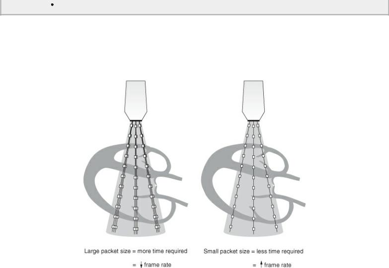
The number of times a line of sound is sampled is referred to as its packet size (Figure 1.34). Increasing packet size improves image quality and fills in the color display, but this is at the expense of frame rate. Packet sizes can be selected by the operator on some equipment. Decreasing packet size will increase your frame rate but decrease sampling time. Information may be lost with very short sampling times. This may be necessary however with rapid heart rates. Increasing packet size will increase the time required for sampling and decrease the frame rate, but it will be able to map velocities and color with greater color filling.

Optimize CF Imaging

Decrease transducer frequency.

Decrease color sector width.

Eliminate real-time image.

Increase packet size.

Decreases frame rate however.

Decrease packet size.

Decreases sampling time and good for high heart rates but may lose information.

Figure 1.34 Packet size is the number of times each line within a color sector is sampled. Large packet sizes produce better color images since more samples can be taken. This is at the expense of frame rate, however, since more time is necessary. Smaller packet sizes decrease the number of times each scan line is sampled so color information is not as complete but frame rate is higher.

Tissue Doppler Imaging

Tissue Doppler imaging (TDI) or tissue Doppler echocardiography (TDE) involves acquiring myocardial velocities. While blood cells reflect low amplitude signals at high velocity, myocardial motion has high-amplitude signals but low velocity. Standard Doppler interrogation of blood flow filters out low velocity signals. TDI however bypasses the low velocity filter. TDI can employ pulsedwave signals only or can be used in conjunction with color-flow Doppler. Color TDI uses a narrow sector of color (to keep frame rates high) placed over a section of myocardium. A pulsed-wave gate can be placed anywhere over the color sector after the fact from stored video loops (Figure 1.35). When using pulsed-wave Doppler TDI, the spectral gate is placed over a color Doppler sector in the area of interest on the myocardium and a spectral trace of myocardial motion is displayed in real time (Figure 1.36). The advantage to color TDI is that myocardium anywhere under the color sector can be interrogated after the fact all at the same time and compared. Pulsed-wave TDI is limited to recording myocardial velocities taken in real time under the gate. Pulsed-wave TDI however provides the highest temporal and velocity range resolution.

Figure 1.35 Color-tissue Doppler uses a narrow sector of color placed over myocardium. Here color is placed over the middle of a transverse left ventricular image. Off line analysis allows gates to be placed over the myocardium anywhere within the color sector. Myocardial velocity corresponding to the selected gate or gates is displayed.