

Two-Dimensional Imaging Controls
Introduction
Most ultrasound equipment comes with installed presets that define a set of imaging parameters to optimize image quality for either the size of the animal or the species. These are good starting points and may be perfect for the heart being imaged, but sometimes image quality is less than desired. What follows is a discussion of controls common to all ultrasound equipment that can be adjusted in order to improve image quality when the presets don’t seem to do the job. Refer to your owner’s manual for more detailed information and discussion of options specific to your equipment.
Depth
Depth controls adjust the field of view. Adjust the depth setting until the real-time image fills the field in order to reduce the amount of lung field and reverberation artifact seen at the bottom of the sector. A cursor or other calibration system is typically displayed alongside the sector image (Figure 2.85). Each mark usually represents 1 centimeter of depth.
Figure 2.85 Depth can be adjusted in order to (A) enlarge or (B) decrease the field of view. A scale is displayed on the side of the sector image. Each mark typically represents a centimeter (arrow). LV = left ventricle, IVS = interventricular septum.

Gain
Gain is often called power or transmits on some machines. Gain controls the transducer’s output power or signal strength. The entire sector image is affected by this control. Too high of a gain setting will produce a very white distorted image while too low of a setting will not produce a signal with enough strength to generate a good image (Figure 2.86). Set the gain so the image is clearly seen with no “blooming” of pixels and the chambers contain no extraneous echoes.
Figure 2.86 Gain controls the signal strength for the entire sector image. Here the gain is set too high producing a very white image with “blooming” of pixels and too many echoes within the cardiac chambers. RA = right atrium, IVS = interventricular septum, LV = left ventricle, LA = left atrium, AO = aorta.

Time Gain Compensation
Time gain compensation (TGC) levers control the gain settings at specific depths on the real-time image (Figure 2.87). Gain is increased by sliding the lever to the right and decreased by sliding the lever to the left. This allows the stronger reflections from near-field structures to be toned down (attenuated) while deeper structures that reflect weaker sound can be intensified on the monitor. The levers on the TGC curve should all be in a smooth line—straight or curved. No one lever should be out of the line to the left or right. If an area of increased echogenicity or decreased echogenicity extends across the entire width of the sector image and is limited to a centimeter or 2 of depth on the image, the TCG curve may have a lever moved too far to the right or left (Figure 2.88).
Figure 2.87 Each time gain compensation (TGC) lever (arrow) controls the gain level at specific depths on the sector image. Moving the lever to the right will increase the intensity of the display while moving the lever to the left will attenuate the magnitude of gain on the displayed image.
Typically there is a slight angle of the TGC sliders to the right as depth increases in order to amplify those echoes. No slider should be out of alignment with the one above or below it.

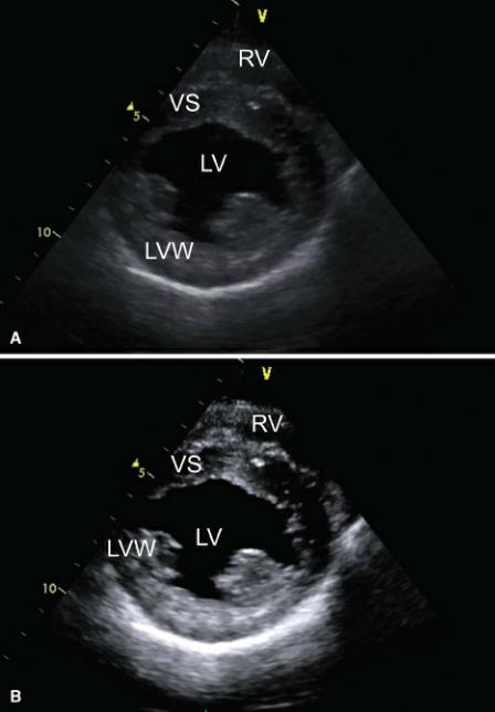
Figure 2.88 This image shows a black streak (arrow) in the middle of the two -dimensional image. It crosses the entire sector and occurs because one sliding lever is too far to the left (attenuating the displayed sound) and out of alignment with the others. RV = right ventricle, LV = left ventricle, VS = ventricular septum, LVW = left ventricular wall.
Compress/Dynamic Range
Compression, called dynamic range on some equipment, adjusts the range of gray on the displayed image. Decreasing the compression level allows weaker echoes to be displayed and more shades of gray are visible. A softer-looking image is created. Increasing compression reduces the dynamic range, eliminates the display of grays associated with weaker signals, results in a higher contrast image, and reduces background noise (Figure 2.89). This is often personal preference but can enhance image quality in difficult to image patients.
Figure 2.89 Compression increases or decreases the number of gray shades displayed in the image. (A) Low compression allows more grays to be displayed, (B) more compression creates an image with less grays and more contrast. RV = right ventricle, VS = ventricular septum, LV = left ventricle, LVW = left ventricular wall.
Persistence/Frame Averaging
This control averages imaging frames by mixing information from old frames with new frames,

resulting in a smoother image with less speckling. Cardiac imaging generally employs little, if any persistence, since the real-time effect becomes blurred with frame averaging.
Sector Width
Sector widths are typically adjustable from about a 120° angle to a narrow width of less than 30° (Figure 2.90). The smaller the sector angle the faster the frame rate and the higher the resolution of the real-time image.
Figure 2.90 Small sector widths (A) increase the frame rate since less sampling time is required, producing a higher resolution image than when larger sector angles (B) are selected.
Focus
Sound beams are narrowed at the level of the focal point enhancing lateral resolution. Place the focal point at the depth level of interest on the ultrasound image. More than one focal point can be set that increases the area of resolution but decreases frame rate because of the time involved in focusing the image. Cardiac imaging usually uses no more than one focal point.
Harmonics
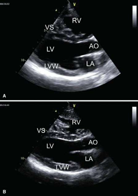
When ultrasound is transmitted at one frequency and returned at twice the transmitted frequency, it is called tissue harmonic imaging. This imaging mode is used to enhance the definition of endocardial borders and reduces the generation of artifacts, especially in patients with poor acoustic windows. The harmonic frequencies are created within the thorax and not at the chest wall where many annoying artifacts originate, and turning harmonics on alleviates many of these imaging artifacts. It also enhances contrast resolution of the ultrasound image. This simple control is easy to turn on and off; on some machines it is a push of a button, on others it involves reducing the transmitting frequency. It is worth remembering to try it when image quality is poor (Figure 2.91).
Figure 2.91 Harmonic tissue imaging uses second and third harmonic reflections that have a higher frequency and thus a higher resolution image in most cases. (A) Harmonics off, (B) harmonics on. RV = right ventricle, VS = ventricular septum, LV = left ventricle, AO = aorta, LA = left atrium, LVW = left ventricular wall.
Gray Map
Echoes returning from tissues are assigned a shade of gray based upon their signal strength (amplitude). Different gray maps assign more or less gray to an image. Maps with less gray lump a range of signal strengths together and assign one gray shade to that range resulting in an image with more contrast than an image that uses a gray map with a greater range of grays. This is usually a postprocessing button on the machine that allows adjustment of gray maps on a frozen or stored image. A different map may enhance a lesion that is difficult to detect with the preset gray map. A different gray map may also enhance the image quality in an animal that is difficult to scan.
References
1. Thomas WP, Gaber CE, Jacobs GJ, et al. Recommendations for standards in transthoracic twodimensional echocardiography in the dog and cat. Echocardiography Committee of the Specialty of Cardiology, American College of Veterinary Internal Medicine. J Vet Intern Med 1993;7:247–252.
2.O’Grady M, Bonagura J, Powers J, et al. Quantitative cross-sectional echocardiography in the normal dog. Vet Rad Ultra 1986;27:34–49.
3.Schiller N, Skiôldebrand C, Schiller E, et al. Canine left ventricular mass estimation by twodimensional echocardiography. Circ 1983;68:210–216.
4.Thomas W. Two-dimensional, real-time echocardiography in the dog: technique and anatomic validation. Vet Rad 1984;25:50–64.
5.Bonagura J, O’Grady M, Herring D. Echocardiography: principles of interpretation. Vet Clin N Am Eq Prac: Sm An Prac 1985;15:1177–1194.
6.Lusk R, Ettinger S. Echocardiographic techniques in the dog and cat. J Am An Hosp Assoc 1990;26:473–488.
7.DeMadron E, Bonagura J, Herring D. Two-dimensional echocardiography in the normal cat. Vet Rad 1985;26: 149–158.
8.Voros K, Holmes J, Gibbs C. Measurement of cardiac dimensions with two-dimensional echocardiography in the living horse. Eq Vet J Suppl 1991;23:461– 465.
9.Long K, Bonagura J, Darke P. Standardized imaging technique for guided m-mode and Doppler echocardiography in the horse. Eq Vet J 1992;24:226–235.
10.Reef V. Echocardiographic examination in the horse: the basics. Compendium 1990;12:1312–1320.
11.Carlsten J. Two-dimensional, real-time echocardiography in the horse. Vet Rad 1987;28:76–87.
12.Voros K, Holmes J, Gibbs C. Anatomical validation of two-dimensional echocardiography in the horse. Equine Vet J 1990;22:392–397.
13.Reimer J. Cardiac evaluation of the horse: using ultrasonography. Vet Med 1993;88:748–755.
14.Stadler P, Rewel A, Deegen E. M-mode echocardiography in dressage and show jumping horses of class “S” and in untrained horses. J Vet Med A 1993;40:292–306.
15.Yamaga Y, Too K. Diagnostic ultrasound imaging in domestic animals: two-dimensional and m- mode echocardiography. Jpn J Vet Sci 1984;46:493–503.
16.Thomas W, Gaber C, Jacobs G, et al. Recommendations for standards in transthoracic twodimensional echocardiography in the dog and cat. J Vet Int Med 1993;7:247–252.
17.Boon J, Wingfield W, Miller C. Echocardiographic indices in the normal dog. Vet Rad Ultra 1983;24:214–221.
18.Hallowell GD, Potter TJ, Bowen IM. Methods and normal values for echocardiography in adult dairy cattle. Journal of Veterinary Cardiology 2007;9:91–98.
19.Patteson M, Gibbs C, Wotton P, et al. Echocardiographic measurements of cardiac dimensions and indices of cardiac function in normal adult thoroughbred horses. Eq Vet J Suppl 1995;19:18–27.
20.Young M, Magid N, Wallereson D, et al. Echocardiographic left ventricular mass measurement in small animals: anatomic validation in normal and aortic regurgitant rabbits. Am J Noninvas Cardiol 1990;4:145–153.
21.Huml R. Radiography corner: tables for echocardiography and abdominal ultrasonography. Vet Tech 1994;15: 170–171.
22.Lombard C. Normal values of the canine m-mode echocardiogram. Am J Vet Res 1984;45:2015– 2018.
23.Schummer A, Wilkens H, Vollmerrhaus B, et al. The Anatomy of the Domestic Animals: The
Circulatory System, the Skin, and the Cutaneous Organs of the Domestic Mammals. Berlin: Verlag Paul Perry, 1981.
24. Tomita H, Arakaki Y, Ono Y, et al. Imbalance of cusp width and aortic regurgitation associated with aortic cusp prolapse in ventricular septal defect. Jpn Circ J 2001;65:500–504.