vk.com/club152685050 | vk.com/id446425943

Setup and Solution

b. Click OK to close the Wall dialog box.

15.4.7. Setting the Operating Conditions

1.	Physics → Solver → Operating Conditions...

a.Enter 10000 Pa for Operating Pressure.

b.Enable Gravity.

The dialog box will expand to show related gravitational inputs.

c.Enter 9.81 m/s2 for Gravitational Acceleration in the Z direction.

d.Enter 303 K for Operating Temperature.

e.Click OK to close the Operating Conditions dialog box.

The Operating Conditions dialog box can be accessed from the Cell Zone Conditions task page.

Release 2019 R1 - © ANSYS,Inc.All rights reserved.- Contains proprietary and confidential information
of ANSYS, Inc. and its subsidiaries and affiliates.	527

vk.com/club152685050Modeling Surface Chemistry| vk.com/id446425943

15.4.8. Simulating Non-Reacting Flow

1.Disable Volumetric for solving non-reacting flow.

Physics → Models → Species...

a.Disable Volumetric in the Reactions group box.

b.Click OK to close the Species Model dialog box.

You will first run a non-reacting solution to establish the flow.

2. Select the Coupled solver method.

Solution → Solution Methods

	Release 2019 R1 - © ANSYS,Inc.All rights reserved.- Contains proprietary and confidential information
528	of ANSYS, Inc. and its subsidiaries and affiliates.

vk.com/club152685050 | vk.com/id446425943

Setup and Solution

Retain the default selections.

3.Enable residual plotting during the calculation.

Solution → Reports → Residuals...

a. Retain the default settings and close the Residual Monitors dialog box.

4.Initialize the flow field.

Solution → Solution Initialization

Release 2019 R1 - © ANSYS,Inc.All rights reserved.- Contains proprietary and confidential information
of ANSYS, Inc. and its subsidiaries and affiliates.	529

vk.com/club152685050Modeling Surface Chemistry| vk.com/id446425943

a.Retain the default selection of Hybrid Initialization from the Initialization Methods group box.

b.Click Initialize.

5.Save the case file (surface-non-react.cas.gz).

File → Write → Case...

6.Start the calculation by requesting 200 iterations.

Solution → Run Calculation

a. Enter 200 for No. of Iterations and click Calculate.

15.4.9. Simulating Reacting Flow

1.Enable Volumetric for the reacting flow solution.

Physics → Models → Species...

	Release 2019 R1 - © ANSYS,Inc.All rights reserved.- Contains proprietary and confidential information
530	of ANSYS, Inc. and its subsidiaries and affiliates.

vk.com/club152685050 | vk.com/id446425943

Setup and Solution

a.Enable Volumetric and Wall Surface in the Reactions group box.

b.Ensure that Mass Deposition Source is enabled in the Wall Surface Reaction Options group box.

c.Click OK to close the Species Model dialog box.

2.Retain the default convergence criteria for calculation.

Solution → Reports → Residuals...

Release 2019 R1 - © ANSYS,Inc.All rights reserved.- Contains proprietary and confidential information
of ANSYS, Inc. and its subsidiaries and affiliates.	531

vk.com/club152685050Modeling Surface Chemistry| vk.com/id446425943

3.Request 200 more iterations.

Solution → Run Calculation → Calculate

4.Compute the mass fluxes.

Results → Reports → Fluxes...

a.Retain the default selection of Mass Flow Rate in the Options group box.

b.Select outlet, velocity-inlet, and wall-4 from the Boundaries selection list.

	Release 2019 R1 - © ANSYS,Inc.All rights reserved.- Contains proprietary and confidential information
532	of ANSYS, Inc. and its subsidiaries and affiliates.

vk.com/club152685050 | vk.com/id446425943

Setup and Solution

In order to properly assess the mass balance, you must account for the mass deposition on the spinning disk. Hence you select wall-4 in addition to the inlet and outlet boundaries.

c.Click Compute, examine the values displayed in the Results and Net Results boxes, and close the Flux Reports dialog box.

The net mass imbalance should be a small fraction (for example, 0.5% or less) of the total flux through the system. If a significant imbalance occurs, you should decrease your residual tolerances by at least an order of magnitude and continue iterating.

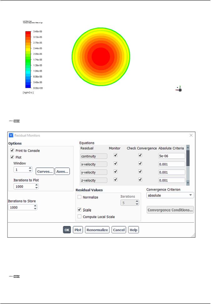
5.Display contours of surface deposition rate of ga (Figure 15.3: Contours of Surface Deposition Rate of Ga (p. 534)).

Results → Graphics → Contours → Edit...

a.Enable Filled in the Options group box.

b.Select Species... and Surface Deposition Rate of ga from the Contours of drop-down lists.

c.Select wall-4 from the Surfaces selection list.

d.Click Display and close the Contours dialog box.

Rotate the display with the mouse to obtain the view as shown in (Figure 15.3: Contours of Surface De- position Rate of Ga (p. 534)).

Release 2019 R1 - © ANSYS,Inc.All rights reserved.- Contains proprietary and confidential information
of ANSYS, Inc. and its subsidiaries and affiliates.	533

vk.com/club152685050Modeling Surface Chemistry| vk.com/id446425943

Figure 15.3: Contours of Surface Deposition Rate of Ga

6.Reduce the convergence criteria.

Solution → Reports → Residuals...

a.Enter 5e-06 for Absolute Criteria for continuity.

b.Click OK to close the Residual Monitors dialog box.

7.Request 200 more iterations.

Solution → Run Calculation → Calculate

	Release 2019 R1 - © ANSYS,Inc.All rights reserved.- Contains proprietary and confidential information
534	of ANSYS, Inc. and its subsidiaries and affiliates.

vk.com/club152685050 | vk.com/id446425943	Setup and Solution
Figure 15.4: Scaled Residuals

8.Check the mass fluxes.

Results → Reports → Fluxes...

a.Retain the default selection of Mass Flow Rate in the Options group box.

b.Retain the selection of outlet and velocity-inlet and, wall-4 from the Boundaries selection list.

c.Click Compute, examine the values displayed in the Results and Net Results boxes, and close the Flux Reports dialog box.

Again, the net mass imbalance should be a small fraction (for example, 0.5% or less) of the total flux through the system.

9.Save the case and data files (surface-react1.cas.gz and surface-react1.dat.gz).

Release 2019 R1 - © ANSYS,Inc.All rights reserved.- Contains proprietary and confidential information
of ANSYS, Inc. and its subsidiaries and affiliates.	535