vk.com/club152685050Using a Single Rotating Reference| vk.com/id446425943Frame

a.Select velocity-inlet-2 and pressure-outlet-3 from the Boundaries selection list.

b.Retain the default Mass Flow Rate option.

c.Click Compute and close the Flux Reports dialog box.

Warning

The net mass imbalance should be a small fraction (for example, 0.5%) of the total flux through the system. If a significant imbalance occurs, you should decrease the residual tolerances by at least an order of magnitude and continue iterating.

9. Save the case and data files (disk-ke.cas.gz and disk-ke.dat.gz).

File → Write → Case & Data...

Click OK to overwrite disk-ke.cas.gz.

Note

It is always prudent to save both case and data files in case anything has changed.

9.4.9. Postprocessing for the Standard k- ε Solution

1.Display the velocity vectors.

Results → Graphics → Vectors → Edit...

	Release 2019 R1 - © ANSYS,Inc.All rights reserved.- Contains proprietary and confidential information
336	of ANSYS, Inc. and its subsidiaries and affiliates.

vk.com/club152685050 | vk.com/id446425943

Setup and Solution

a.Enter 1 for Scale

b.Set Skip to 1.

c.Click the Vector Options... button to open the Vector Options dialog box.

i.Disable Z Component.

This allows you to examine only the non-swirling components.

ii.Click Apply and close the Vector Options dialog box.

Release 2019 R1 - © ANSYS,Inc.All rights reserved.- Contains proprietary and confidential information
of ANSYS, Inc. and its subsidiaries and affiliates.	337

vk.com/club152685050Using a Single Rotating Reference| vk.com/id446425943Frame

d.Click Display in the Vectors dialog box to plot the velocity vectors.

A magnified view of the velocity field displaying a counter-clockwise circulation of the flow is shown in Figure 9.4: Magnified View of Velocity Vectors within the Disk Cavity (p. 338).

Figure 9.4: Magnified View of Velocity Vectors within the Disk Cavity

e.Close the Vectors dialog box.

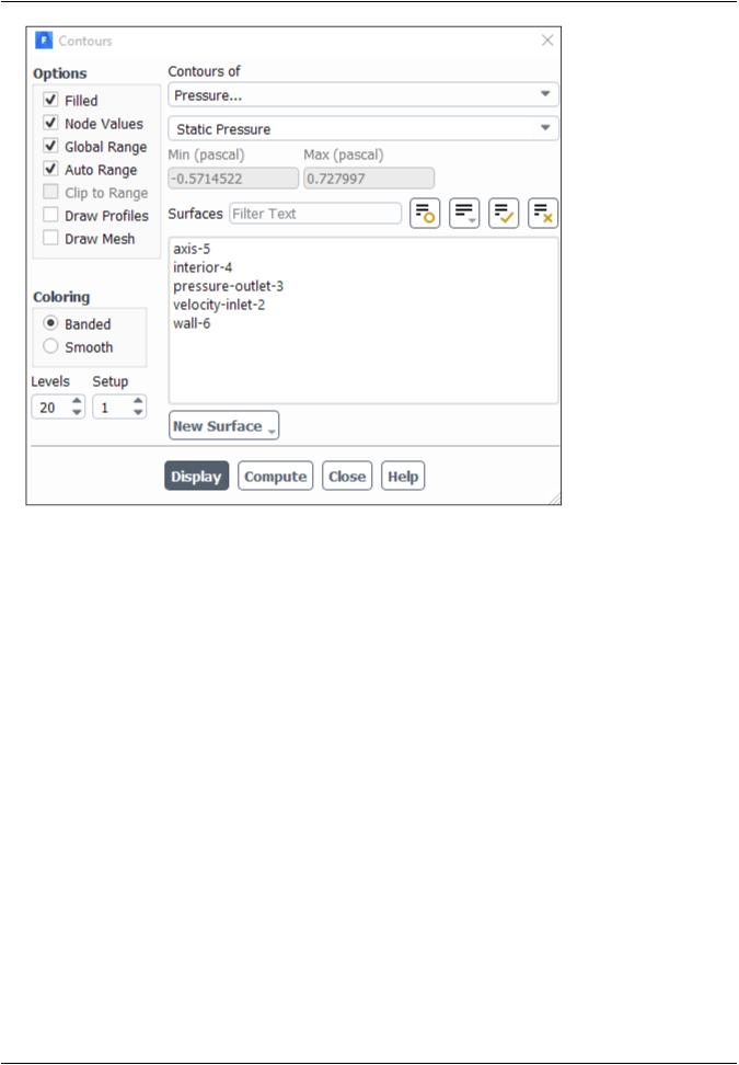
2.Display filled contours of static pressure.

Results → Graphics → Contours → Edit...

	Release 2019 R1 - © ANSYS,Inc.All rights reserved.- Contains proprietary and confidential information
338	of ANSYS, Inc. and its subsidiaries and affiliates.

vk.com/club152685050 | vk.com/id446425943

Setup and Solution

a.Enable Filled in the Options group box.

b.Retain the selection of Pressure... and Static Pressure from the Contours of drop-down lists.

c.Click Display and close the Contours dialog box.

The pressure contours are displayed in Figure 9.5: Contours of Static Pressure for the Entire Disk Cav- ity (p. 340). Notice the high pressure that occurs on the right disk near the hub due to the stagnation of the flow entering from the bore.

Release 2019 R1 - © ANSYS,Inc.All rights reserved.- Contains proprietary and confidential information
of ANSYS, Inc. and its subsidiaries and affiliates.	339

vk.com/club152685050Using a Single Rotating Reference| vk.com/id446425943Frame

Figure 9.5: Contours of Static Pressure for the Entire Disk Cavity

3.Create a constant -coordinate line for postprocessing.

Results → Surface → Create → Iso-Surface...

a.Enter aaa_y=37cm for the New Surface Name.

Using a prefix such as aaa or zzz allows you to keep all postprocessing surfaces together.

b.Select Mesh... and Y-Coordinate from the Surface of Constant drop-down lists.

c.Click Compute to update the minimum and maximum values.

	Release 2019 R1 - © ANSYS,Inc.All rights reserved.- Contains proprietary and confidential information
340	of ANSYS, Inc. and its subsidiaries and affiliates.

vk.com/club152685050 | vk.com/id446425943

Setup and Solution

d.Enter 37 in the Iso-Values field.

This is the radial position along which you will plot the radial velocity profile.

e.Enter aaa_y=37cm for the New Surface Name.

Using a prefix such as aaa or zzz allows you to keep all postprocessing surfaces together.

f.Click Create to create the isosurface.

Note

The name you use for an isosurface can be any continuous string of characters (without spaces).

g.Close the Iso-Surface dialog box.

4.Plot the radial velocity distribution on the surface aaa_y=37cm.

Results → Plots → XY Plot → Edit...

a.Select Velocity... and Radial Velocity from the Y Axis Function drop-down lists.

b.Select the y-coordinate line aaa_y=37cm from the Surfaces selection list.

c.Click Plot.

Figure 9.6: Radial Velocity Distribution—Standard k- ε Solution(p. 342) shows a plot of the radial velocity distribution along .

Release 2019 R1 - © ANSYS,Inc.All rights reserved.- Contains proprietary and confidential information
of ANSYS, Inc. and its subsidiaries and affiliates.	341

vk.com/club152685050Using a Single Rotating Reference| vk.com/id446425943Frame

Figure 9.6: Radial Velocity Distribution—Standard k- ε Solution

d.Enable Write to File in the Options group box to save the radial velocity profile.

e.Click the Write... button to open the Select File dialog box.

i.Enter ke-data.xy in the XY File text entry box and click OK.

Be sure to double check the location where the files are being saved to ensure they will be saved where you intend.

5.Plot the wall y+ distribution on the rotating disk wall along the radial direction (Figure 9.7: Wall Yplus Distribution on wall-6— Standard k- ε Solution (p. 344)).

Results → Plots → XY Plot → Edit...

	Release 2019 R1 - © ANSYS,Inc.All rights reserved.- Contains proprietary and confidential information
342	of ANSYS, Inc. and its subsidiaries and affiliates.

vk.com/club152685050 | vk.com/id446425943

Setup and Solution

a.Disable Write to File in the Options group box.

b.Select Turbulence... and Wall Yplus from the Y Axis Function drop-down lists.

c.Deselect aaa_y=37cm and select wall-6 from the Surfaces selection list.

d.Enter 0 and 1 for X and Y respectively in the Plot Direction group box.

Note

The change in Plot Direction is required because we are plotting y+ along the radial dimension of the disk, which is oriented with Y axis.

e. Click the Axes... button to open the Axes - Solution XY Plot dialog box.

Release 2019 R1 - © ANSYS,Inc.All rights reserved.- Contains proprietary and confidential information
of ANSYS, Inc. and its subsidiaries and affiliates.	343

vk.com/club152685050Using a Single Rotating Reference| vk.com/id446425943Frame

i.Retain the default selection of X from the Axis group box.

ii.Disable Auto Range in the Options group box.

iii.Retain the default value of 0 for Minimum and enter 43 for Maximum in the Range group box.

iv.Click Apply and close the Axes - Solution XY Plot dialog box.

f.Click Plot in the Solution XY Plot dialog box.

Figure 9.7: Wall Yplus Distribution on wall-6— Standard k- ε Solution(p. 344) shows a plot of wall y+ distribution along wall-6.

Figure 9.7: Wall Yplus Distribution on wall-6— Standard k- ε Solution

	Release 2019 R1 - © ANSYS,Inc.All rights reserved.- Contains proprietary and confidential information
344	of ANSYS, Inc. and its subsidiaries and affiliates.